Thermal fluctuation fields in basalts
Adrian R. Muxworthy1, David Heslop2, and Daniel M. Michalk3
1Department of Earth Sciences and Engineering, Imperial College London, South Kensington Campus, London, SW7 2AZ, UK 2Fachbereich Geowissenschaften, Universit¨at Bremen, Klagenfurter Straße, 28359 Bremen, Germany
3GeoForschungsZentrum Potsdam, Section 3.3, Telegrafenberg, 14473 Potsdam, Germany
(Received September 4, 2007; Revised January 23, 2008; Accepted January 25, 2008; Online published January 23, 2009)
The thermal fluctuation field (Hf) is central to thermoremanent acquisition models, which are key to our
understanding of the reliability of palaeomagnetic data, however, Hf is poorly quantified for natural systems.
We reportHf determinations for a range of basalts, made by measuring rate-dependent hysteresis. The results
for the basalts were found to be generally consistent within the space ofHf versus the coercive force HC, i.e.,
the “Barbier plot”, which is characterized by the empirically derived relationship; logHf ∝1.3 logHCobtained
from measurements on a wide range of different magnetic materials. Although the basalts appear to occupy the correct position within the space of the Barbier plot, the relationship within the sample set, logHf∝0.54 logHC,
is different to the Barbier relationship. This difference is attributed to the original Barbier relationship being derived from a wide range of different synthetic magnetic materials, and not for variations within one material type, as well as differences in methodology in determiningHf. We consider the relationship betweenHCand the
activation volume,vact, which was found to beHC∝v−act0.68for our mineralogically homogeneous samples. This
compares favourably with theoretical predictions, and with previous empirical estimates based on the Barbier plot, which defined the relationship asHC∝vact−0.73.
Key words:Basalt, thermoremanence, thermal fluctuations, rock magnetism.
1.
Introduction
N´eel (1950, 1951) introduced the concept of a thermal fluctuation (or viscosity) field to describe the influence of thermal fluctuations on a magnetic system. This abstract concept is very powerful, as it allows for a magnetic sys-tem’s behaviour to be entirely described in terms of mag-netic fields. Thermal fluctuations influence all thermally activated magnetic processes, i.e., for temperaturesT > 0 K, becoming increasingly important for magnetisation pro-cesses at high or variable temperatures, such as thermore-manence (TRM) acquisition. As such the concept of ther-mal fluctuation fields are central to many theories of both single-domain (SD) and multidomain (MD) TRM acquisi-tion, on which many palaeomagnetic concepts and method-ologies are based, e.g., the Thellier and Thellier (1959) method and its modifications for palaeointensity determi-nation.
In the literature there are several definitions for thermal fluctuation or viscosity fields. In this paper we use the definition for the thermal fluctuation field, Hf, described
by Wohlfarth (1984), which has subsequently been used widely in the physics literature. Wohlfarth’s description is based on the work of N´eel (1950, 1951) and Street and co-workers (Street and Woolley, 1949, 1950; Streetet al., 1952; Street and Woolley, 1956), and relatesHfto the
mag-netic viscosity parameterSand to the irreversible
suscepti-Copyright cThe Society of Geomagnetism and Earth, Planetary and Space Sci-ences (SGEPSS); The Seismological Society of Japan; The Volcanological Society of Japan; The Geodetic Society of Japan; The Japanese Society for Planetary Sci-ences; TERRAPUB.
bilityχirrby the equation:
S=χirrHf (1)
This equation is valid because Hf is related to relaxation
events due to irreversible barrier hopping.
In selected literature the Hf term has been previously
referred to as SV (e.g., Barbier, 1954; Bina and Pr´evot,
1994), but we follow the notation of Wohlfarth (1984) who emphasised that usingSVcan be misleading because it is an
effective field and has different units toS.
It is common to define Hf by relating it to the thermal
activation energy,E, which reduces to (Street and Woolley, 1949; Streetet al., 1952):
E =vactμ0MSHf=kBT
i.e., Hf = kBT vactμ0MS
(2)
wherekB is the Boltzmann’s constant, vact the activation
volume, MS the spontaneous magnetisation of a material
and μ0 the permeability of free space. It is often
as-sumed that vact is identical to the actual volume for
iso-lated “ideal” single domain (SD) grains, and for multido-main (MD) grains the effective volume covered by a sin-gle jump between pinning sites for a domain wall or other such domain wall events (Wohlfarth, 1984; Gaunt, 1986). For SD grains thought to switch via coherent rotation, this conclusion appears to be correct in the case of magnetite and thus magnetic granulometry techniques can be based on the determination of vact (Dunlop, 1976; Dunlop and
Bina, 1977). Studies on interacting particles have shown
that the estimatedvact, is greater than the volume of
indi-vidual magnetic particles (e.g., Bottoni, 2005; El-Hilo and Bsoul, 2007).
As thermal fluctuation fields were introduced by N´eel (1950, 1951) as a “most pictorial concept” (Wohlfarth, 1984), the question arises as to how Hf can be quantified
experimentally. There are basically four broad approaches to determiningHf; (1) by measuring the time dependency
of remanent or induced magnetisation, e.g., viscous decay curves (Sholpo, 1967; Bina and Pr´evot, 1994; El-Hiloet al., 2002), (2) by determining the time dependency of hystere-sis, e.g., variable field-sweep-rate hysteresis (Brunoet al., 1990), (3) by examining alternating field demagnetisation curves (Pr´evot, 1981; Bina and Pr´evot, 1994) and (4) by measuring magnetic behaviour as a function of temperature (Dunlop, 1976).
Each of these methods is based on certain assumptions and approximations and can yield different values for the same samples (e.g., Bina and Pr´evot, 1994). For some cases a method may only be appropriate for a particular domain state, for example, consider the last method; because Hf
is temperature dependent for MD material (Barbier, 1954), this method is only appropriate for coherently switching SD particles.
Barbier (1951, 1954) showed a most surprising linear correlation between logHf and logHC for a range of soft
and hard magnetic materials, yielding the empirical rela-tionship,
logHf≈mlogHC−C (3)
wherem is the gradient andC a constant. Barbier (1951, 1954) found empirical estimates for m andC of 1.3 and
−3.3 respectively. This empirical relationship has been sub-sequently found to be consistent for other materials (Wohl-farth, 1984; Liu and Luo, 1990; Sunet al., 1990; Liu and Luo, 1991; te Lintelo and Lodder, 1994). Using Eq. (2) this leads to the conclusion thatHC∝vact−0.73(Wohlfarth,
1984).
Theoretical models are in slight disagreement with this experimental relationship (e.g., Liu and Luo, 1990, 1991; Klik and Chang, 1992). These models for SD behaviour and various MD pinning mechanisms all predict via Eq. (2) a gradient of unity rather than the empirical value of 1.3, however, these results are based on simplified models for magnetic structure and do not incorporate the more complex micromagnetic structures predicted by numerical models (Williams and Dunlop, 1989) and observed using electron-holography (Mankos et al., 1996), i.e., primarily non-uniform magnetic structures such as vortex-like structures.
As thermal fluctuation fields are central to our theories of natural magnetic remanence (NRM) in igneous and meta-morphic rocks, a thorough understanding and knowledge of their effects in natural magnetic systems is important if we are to be confident of the robustness of palaeomagnetic re-sults and predictions.
There have been numerous studies, which have investi-gated and quantified Hf andvact in synthetic powders
in-cluding magnetite and other minerals of geophysical inter-est (e.g., Shimizu, 1960; Sholpo, 1967; Sholpoet al., 1972; Dunlop, 1976; Dunlop and Bina, 1977), however, there
have been far fewer reports for actual rocks, such as the basalts which are commonly used in palaeomagnetic studies and for palaeointensity determinations (Sholpoet al., 1972; Pr´evot, 1981; Bina and Pr´evot, 1994). Sholpoet al.(1972) determinedHfandvactfor a range of rock types, with
val-ues forHfin the range∼1000–2200 A/m for basalts and up
to∼6400 A/m for sandstones. Pr´evot (1981) and Bina and Pr´evot (1994) determinedHffor two subaerial basalts and
two ocean basalt samples containing maghematized MD ti-tanomagnetite. Using a variety of different methods to de-termineHf, yielded a scatter of values (subaerial basalts: 7–
12 A/m, submarine basalts: 1.8–27 A/m), much lower than those reported by Sholpoet al.(1972) for their basalts. This difference may simply be due to different coercivities of the samples employed in the two studies. The MD submarine samples of Bina and Pr´evot (1994) had coercive fields of just∼2500 A/m. Sholpoet al.(1972) did not reportHCfor
their samples, but using Eq. (3) to estimate HC gives
val-ues of∼34000–75000 A/m for their basalt samples. These are a little higher than is usually observed but possible for highly stressed SD material. The high value may also be related to the method employed (Sholpo, 1967), which is based on viscous decay curves alone, which can yield esti-mates forHf an order of magnitude greater than those
de-rived by other methods for the same samples (pers. comm. M. Pr´evot, 2007).
Pr´evot (1981) and Bina and Pr´evot (1994) found a strong dependence ofHf on temperature for their MD material in
agreement with Barbier (1954).
Thermal fluctuation fields are central to thermoremanent acquisition theories and our understanding of viscosity, yet they are poorly quantified for natural systems, with only a few samples studied to date. In this paper we report a detailed study whose aim is to determine Hf for
natu-ral magnetic systems, in particular basalts, and to exam-ine whether the empirical relationship originally derived by Barbier (1951, 1954) is valid for basalts and thus could be potentially applied to rock magnetic theories.
2.
Samples
Due to the nature of the relationship found by Barbier (1951, 1954), i.e., logHf versus logHC, we required basalt
samples with as wide a range of coercivities as possible. We considered two sets of samples, Pleistocene basalts from Mexico of Brunhes Chron ages (<780 ka), and historical samples from Iceland (1729–2000 AD). These basalt sam-ples had a range of coercivities, varying from a minimum of 2.7 kA/m up to 36 kA/m (Table 1). Some further Mexican samples, characterized by highly wasp-waisted loops, were rejected from this study because they did not saturate dur-ing hysteresis (maximum available field=1600 kA/m). It is thought that these rocks underwent alteration due to trop-ical weathering, which caused low temperature oxidation (maghemitization) of the magnetic carriers.
Table 1. Curie temperature,HC,Hf, andMSpredictions.
Sample name Origin Curie temperature (◦C) HC(kA/m) Hf(A/m) estimatedMS(kA/m)
ab12 CSP (450 ka) 237 2.7 15 178
ad2 CSP (450 ka) 549 36 110 452
br6 VDB 533 9.7 48 436
bs02 VDB 561 22 38 465
bt09 VDB 328 9.5 51 251
bt11 VDB 332 9.7 48 253
bv03 VDB 552 14 26 455
h00h Hekla (2000) 235 3.9 32 177
hc1 Hekla (1845) 120 14 72 92
hd1 Hekla (unknown) 90 22 49 71
hf2 Hekla (unknown) 320 31 110 244
hf5 Hekla (unknown) 320 28 110 244
ka1 Krafla (1981) 90 22 38 71
ka2 Krafla (1981) 90 38 28 71
ka3 Krafla (1981) 90 12 64 71
kb5 Krafla (1729) 110 9.8 64 85
kb9 Krafla (1729) 110 12 46 85
Ceboruco-San Pedro (CSP) and Valle de Bravo (VDB, undated but Brunhes Chron) are two monogenic volcanic fields within the Transmexican Volcanic Belt. Hekla and Krafla are two volcanoes in Iceland, with very recent eruptions. Hekla (unknown) lavas are from undated flows from Hekla, but Brunhes Chron. The Curie temperatures were determined from saturating thermomagnetic curves (heating in Argon). Only the primary or dominant Curie temperature is shown. HCandHfas depicted in Fig. 3 are tabulated. From the primary Curie temperature estimates,MSwas determined assuming
that the variation in Curie temperature was due to titanium variation within titanomagnetite minerals (Huntet al., 1995). The Curie temperatures were determined using a variable field translation balance using an applied continuous field of 500 mT.
SD
H CR /H C
M RS
/M
S
0 1 2 3 4 5 6
0 0. 1 0. 2 0. 3 0. 4 0. 5 0. 6
PSD
MD
-1000 -500 500 1000
-1 1
M/MS
sample HF2
-500 -250 250 500
-1 1
Icel an d Me xico
sample AB12
M/MS field (mT)
field (mT)
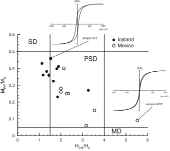
Fig. 1. A “Day plot” (Dayet al., 1977) ofMRS/MSversusHCR/HCfor the Icelandic and Mexican samples considered in this study, whereMRSis
the remanent saturation magnetisation andHCRthe remanent coercive force. The two insets show hysteresis loops for two of the end members. The
Mexican sample AB12 is slightly wasp-waisted.
sub-micron titanomagnetite (C1) and ilmenite (R1) needles. The presence of needles is indicative of fast cooling. The samples from Krafla consisted of small skeletal titanomag-netites (C1) similar to those reported by Kr´asa and Matzka (2007). Curie temperatures determined for the Icelandic
samples ranged from 90 to 320◦C (Table 1).
observations revealed a range of oxidation states and grain sizes. For example, sample AB consisted of a mixture of anhedral and euhedral titanomagnetite grains (C1 oxi-dation state, 10–50 μm in size), some larger grains dis-playing deuteric trellis textures (C3) and a few finer grains within the matrix. The “B” samples, i.e., BR, BS, BT and BV, displayed large grains with cracked rims probably due to maghemitization, with some evidence for high tempera-ture oxyexsolution and fine-grained hematite. The samples also had a wide range of Curie temperatures, varying from 237◦C to 561◦C (Table 1).
3.
Experimental Results
There are several approaches for determining Hf. We
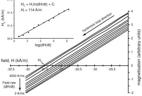
used the rate-dependent hysteresis method proposed by Brunoet al.(1990). This requires measuring the coerciv-ity as a function of field rate, i.e.,d H/dt, where H is the applied field andt the time. Hf is then given by (Brunoet al., 1990; Bassoet al., 2000),
HC=Hflog(d H/dt)+C (4)
whereC, according to theory, is constant for a given tem-perature (Bruno et al., 1990). It might be argued that palaeomagnetists are more commonly interested in ther-mal activation of remanent magnetisation rather than dur-ing hysteresis, that is, it might be more appropriate to use viscous decay of remanence curves to determine Hf if the
findings are to be applied to palaeomagnetic investigations. We chose to measure Hf using this in-field hysteresis
ap-proach, as it yields significantly improved signal-to-noise ratios compared to measurement of viscous decay of rema-nent magnetisation.
We measured Hf as a function of field rate using a
Princeton Measurements alternating gradient magnetome-ter (AGM), with rates from∼2 to∼4000 A m−1s−1. The
hysteresis loops were measured in an automated sequence requiring several hours to complete. A number of steps were taken to reduce and accommodate instrument drift, including off resonance-peak measurements and repeated intermediate measurements to allow drift correction. All measurements were made at room temperature and the in-strument drift was assumed to be linear with respect to time. An example ofHfdetermination is shown in Fig. 2. As
ex-pected from Eq. (4),HCis seen to increase in a linear
man-ner with respect to log(d H/dt).
The values of Hf of the individual samples and their
relationship withHCwere determined using a Monte Carlo
procedure based on bootstrapping the measured hysteresis data (Efron and Tibshirani, 1993). Each iteration of the Monte Carlo procedure involved the following sequence of steps:
Step 1. The log(d H/dt)versus HC data for each sample
was bootstrapped (with replacement) to form an esti-mate ofHffor each sample.
Step 2. Based upon regression, the obtained values of Hf
were used to make an estimate of the linear relation-ship between logHCand logHf.
The above procedure was repeated for 104trials and the
dis-tribution of results for each step could be used to estimate
30.6
Fig. 2. A typical example of the measurement of field-rate dependent hysteresis, and the variation in coercive force HC. The inset shows
howHfwas determined from such hysteresis data. The sample is the
Icelandic sample hf2.
the discussed parameters with associated confidence inter-vals. Step 1 of the procedure was used to estimateHfwithin
90% confidence limits for each of the samples. The collec-tion of regression equacollec-tions determined in step 2 yielded an estimate for the linear relationship between logHf and
logHCwithin a 90% region of confidence (Fig. 3(a)), where
logHCwas defined using the fastest measuring rate in
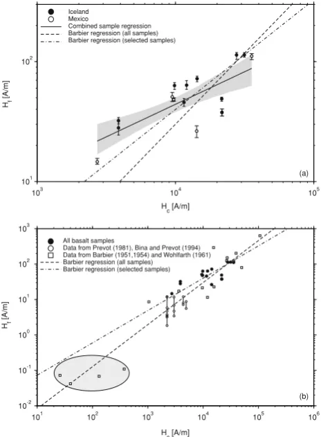
or-der to minimize the effects of thermal fluctuation (Fig. 2). It was found that as a first approximation the basalts can be fitted by the relationship logHf≈0.54 logHC−0.52. HC
andHfare tabulated in Table 1.
4.
Discussion
When the basalt data from this study is plotted with the original “Barbier data” (which includes the data of Barbier (1951, 1954) and Wohlfarth (1961), Fig. 3(b)), it is seen that the basalt data lies on the overall trend of the Barbier data. When, however, the gradient of the basalt data is de-termined using Eq. (3) it is found to be substantially lower than that of the Barbier data set, i.e., 0.54 versus 1.3 re-spectively. There are a number of possible reasons for this; first—and we suggest the most important point—the origi-nal fit to the Barbier data essentially examines behavioural trends between a wide range of different materials, whereas, although the basalts examined have a variety of composi-tions, they are essentially the “same” material, i.e., titano-magnetites with varying degree of oxidation. In this way we are applying Eq. (3) in two different forms; for a range of materials in the case of the Barbier data and within a sin-gle material for the basalt samples. Second, the range for the Barbier data is much wider than for the basalt data set. Third, different methods have been employed to determine
Hf; the method utilised in this paper determinesHfat higher
fields than the viscous decay mechanisms;Hfis determined
101 102 103 104 105 106
Data from Barbier (1951,1954) and Wohlfarth (1961) Barbier regression (all samples)
from Prevot (1981), Bina and Prevot (1994)
Barbier regression (selected samples)
(a)
(b)
Fig. 3. (a) Plot of logHfversus logHC, i.e., a Barbier plot, for the
Ice-landic and Mexican samples considered in this study, the error bars on each point represent the 90% confidence interval obtained using the Monte Carlo procedure described in the text. The Monte Carlo pro-cedure also yielded an estimate of the relationship (solid black line) between logHfand logHCand is shown with a 90% confidence region
(shaded area). In addition we show two further regression lines, the first (dashed line) is based on the full “Barbier data set” (Barbier (1951, 1954 #21940) and Wohlfarth (1961)) and the second (dot-dashed line) is cal-culated from the same data with the low coercivity materials removed. (b) Plot of logHfversus logHCfor the basalts measured in this study
(filled circles), the “Barbier data” (open squares), plus trend lines for the Barbier and reduced Barbier data sets. As in panel (a) the former line is fitted to all the Barbier data, the latter to Barbier data minus the strongly biasing very lowHCsamples, which are highlighted in the figure with
a shaped ellipse. The data of Pr´evot (1981) and Bina and Pr´evot (1994) for four samples, are shown as a range of values (open circles with con-necting lines) based on the variety of methods they employed to estimate
Hf.
potentially leading to a lower gradient in Fig. 3. Fifth, the regression of the Barbier data set is heavily influenced by four data points at very low HC values which exert a
sub-stantial leverage on the fit (highlighted in Fig. 3(b)). If these four data points are removed from the regression (Fig. 3), then the gradient is reduced and the new slope plots closer to the basalt data regression line. This alternative fit to the Barbier data, which is restricted to higher coercivity mate-rials, passes through the centre of the basalt data and thus appears to be more appropriate to our sample set.
On Fig. 3(b), the data of Pr´evot (1981) and Bina and Pr´evot (1994) are plotted. Pr´evot (1981) and Bina and Pr´evot (1994) used several different methods to determine
Hf, producing a range of estimates. They did not use the
rate-dependent hysteresis method that was employed in the
current study. It can be seen that for some of their sam-ples, the variation in Hf for a given sample, is greater in
log-space than the whole spectrum of variation in our data (Fig. 3(b)). This makes it difficult to draw detailed compar-isons between the studies, however, it is clear that the low-coercivity Mexican samples in this study have higher Hf
values than reported by Pr´evot (1981) and Bina and Pr´evot (1994). This difference maybe due to the different methods employed to determineHfand/or the apparent bi-modal
co-ercivity distributions of the Mexican samples.
4.1 Activation volumes
The basaltic samples have a wide range of domain states (Fig. 1), coercivities (varying from 2.7 kA/m up to 36 kA/m, Table 1), Curie temperatures (Table 1) and oxidation states, yet all the samples as a first approximation agree with a fit of Eq. (3). This implies that the mechanisms that control the coercivity in both SD and MD grains are affected by thermal fluctuations to the same extent. As stated previously, it is thought that in the smallest grainsvactcorresponds to actual
grain volume, whereas in the larger grains it is related to nucleation volumes and volumes associated with pinning movements. This implies that the same localities, which correspond to switching or reversal processes, are also the same sites that are activated thermally.
Using Eqs. (2) and (3) with the addition of one data point from Wohlfarth (1961) to the plot of Barbier (1954), Wohl-farth (1984) concluded thatHC∝v−actx, withx=0.73. This
relationship has been cited many times (e.g., Liu and Luo, 1991; te Lintelo and Lodder, 1994), yet, it is unclear if Wohlfarth (1984) included the variation ofMS(Eq. (2)) in
his determination; it is apparent that the description of the samples provided in the published work would be insuffi-cient to do this. If the variation in MS is ignored, using
the data available to Wohlfarth (1984) yieldsx=0.74; this small difference inxis likely to be within rounding errors. Theoretical estimates forxdepend on reversal mechanisms, and range from 0.5<x<1 (e.g., N´eel, 1951; Hilzinger and Kronm¨uller, 1975; Liu and Luo, 1990, 1991). It is gener-ally predicted thatx=1 for uniaxial SD particles, but there are several discrepancies between domain wall theories, for example, Liu and Luo (1991) predictx=1 for all reversal mechanisms, in contrast to a lower value of 0.5 by Hilzinger and Kronm¨uller (1975).
Ignoring the variation MSand apply Eq. (2) to our
find-ings for all 17 samples in Fig. 3, yields HC ∝ v−act1.9. To
estimate variations inMS, we assumed that the variations in
Curie temperature (Table 1) are due to titanium substitution. We could only make this assumption for the Icelandic sam-ples, as the Mexico samples displayed visible alteration and oxidation under the microscope. We applied the relation-ships given by Huntet al.(1995) to make predictions forMS
(Table 1). Our estimates of the Curie temperatures are “pri-mary” i.e., the “main” peak of thermomagnetic curves. Two more steps were added to the previously discussed Monte Carlo procedure to evaluatevactfor our basalt samples and
its relationship to logHC:
Step 3. Given the values ofHfcalculated in the first Monte
Carlo step, estimates ofvactwere made for each of the
103 104 105
10-22
10-21
H
c[A/m]
Activation
volume
[m
3]
Iceland Mexico
Combined sample regression
40 60 80 100 120 140 160
Activation
length
[nm]
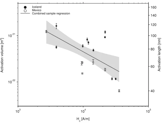
Fig. 4. Logvactversus logHCfor the Icelandic samples. The activation volume was calculated from Eq. (2) using the Monte Carlo procedure described
in the text and employing each sample’s Curie temperature basedMSestimation. The error bars on each point represent the 90% confidence interval,
(Table 1). The Monte Carlo procedure also yielded an estimate of the relationship (solid black line) between logvactand logHCwhich and is shown
with the associated 90% confidence region (shaded area). The activation length, i.e.,v1act/3, is depicted on the right vertical axis for reference.
Step 4. A linear regression was performed between the es-timated values ofvactand logHC.
Estimates ofvact for each sample were made based on the
results of step 3, again with 90% confidence intervals. Fi-nally, the linear relationship betweenvactand logHCwithin
a 90% confidence region was determined from the distribu-tion of results from step 4 (Fig. 4). The Monte Carlo pro-cedure yielded an estimate ofHC∝vact−0.68. This is
consid-erably closer to the value derived by Wohlfarth (1984), and falls within the range of theoretical predictions. Hilzinger and Kronm¨uller (1975) predicted HC ∝vact−2/3 for strongly
pinned domain walls, similarly the Kersten inclusion theory of domain-wall motion also predicts the same relationship (Wohlfarth, 1984).
5.
Conclusions
This is the first time that the relationship found by Bar-bier (1951, 1954) has been measured and tested for natu-ral magnetic systems. The basalt samples were found to agree with the general relationship found by Barbier when compared to other magnetic materials, but the relationship within the basalts themselves is slightly different. Linear re-gression for logHf versus logHCyields a gradient of 0.54
for the basalt samples, compared to the value of 1.3 found when many different materials are considered. This differ-ence is attributed to the fact, that the original relationship by Barbier was derived for a wide range of different syn-thetic magnetic materials, and not for variations within one particular material type.
The relationship between activation volume and coercive force was examined. By considering variation ofMS
esti-mated from measured Curie temperatures, we found for the homogeneous Icelandic basalts, that HC ∝vact−0.68 (Fig. 4).
This falls comfortably in the range of predicted values, i.e., 0.5<x<1, and compares favourably with empirical
find-ing of Wohlfarth (1984) ofHC∝vact−0.73for a wide range of
materials, however, it is unknown if Wohlfarth’s empirical relationship included material variation inMS.
This study provides experimental support for the use of N´eel’s (1950, 1951) thermal fluctuation field in models for TRM acquisition in natural systems. Such theories are key to our under understanding of the reliability of palaeomag-netic data, though the use of the relationship found by Bar-bier should be modified for more appropriate basalt-specific values.
Acknowledgments. We thank Harry Reichard of Princeton Mea-surements Inc. for helping us to develop protocols for perform-ing these measurements on the AGM. ARM would like to Norbert Nowaczyk for the use of the laboratory at the GeoForschungsZen-trum Potsdam. We thank Michel Pr´evot and David Kr´asa for constructive reviews. Fieldwork assistance is gratefully acknowl-edged: Harald B¨ohnel (Mexico) and John MacLennan (Iceland). This work was funded by NERC grant NE/D000351/1, the Royal Society and the DFG.
References
Barbier, J. C., Le traˆınage irr´eversible dans les champs faibles,J. Phys. Rad.,12, 352–354, 1951.
Barbier, J. C., Le traˆınage magn´etique de fluctuation,Ann. Phys.,9, 84– 140, 1954.
Basso, V., C. Beatrice, M. LoBue, P. Tiberto, and G. Bertotti, Connection between hysteresis and thermal relaxation in magnetic materials,Phys. Rev. B,61, 1278–1285, 2000.
Bina, M.-M. and M. Pr´evot, Thermally activated magnetic viscosity in natural multidomain titanomagnetite,Geophys. J. Int.,117, 495–510, 1994.
Bottoni, G., Critical volume for the switching of the magnetization in recording media,J. Magn. Magn. Mater.,272–276, 2269–2270, 2005. Bruno, P., G. Bayreuther, P. Beauvillain, C. Chappert, G. Lugert, D.
Re-nard, J. P. ReRe-nard, and J. Seiden, Hysteresis properties of ultrathin fer-romagnetic films,J. Appl. Phys.,68, 5759–5766, 1990.
Day, R., M. D. Fuller, and V. A. Schmidt, Hysteresis properties of ti-tanomagnetites: grain-size and compositional dependence,Phys. Earth Planet. Inter.,13, 260–267, 1977.
mag-netism,J. Geophys. Res.,81, 3511–3517, 1976.
Dunlop, D. J. and M.-M. Bina, The coercive force spectrum of magnetite at high temperatures: evidence for thermal activation below the blocking temperature,Geophys. J. R. Astr. Soc.,51, 121–147, 1977.
Efron, B. and R. J. Tibshirani,An Introduction to the Bootstrap, 456 pp., Chapman and Hall, New York, 1993.
El-Hilo, M. and I. Bsoul, Interaction effects on the coercivity and fluctu-ation field in granular powder magnetic systems,Physica B,389, 311– 326, 2007.
El-Hilo, M., K. O’Grady, and R. W. Chantrell, Fluctuation fields and reversal mechanisms in granular magnetic systems,J. Magn. Magn. Mater.,248, 360–373, 2002.
Gaunt, P., Magnetic viscosity and thermal activation energy,J. Appl. Phys., 59, 4129–4132, 1986.
Haggerty, S. E., Oxide Textures—A mini-altas, in Reviews in Mineralogy Volume 25—Oxide Minerals, inPetrologic and magnetic significance, edited by D. H. Lindsley, pp. 129–137, Mineralogical Society of Amer-ica, Washington D.C., 1991.
Hilzinger, H. R. and H. Kronm¨uller, Statistical theory of the pinning of Bloch walls by randomly distributed defects,J. Magn. Magn. Mater.,2, 11–17, 1975.
Hunt, C. P., B. M. Moskowitz, and S. K. Banerjee, Magnetic properties of rocks and minerals, inA Handbook of Physical Constants, vol. 3, edited by T. J. Ahrens, pp. 189–204, American Geophysical Union, Washington, DC, 1995.
Klik, I. and C.-R. Chang, A discussion of the Barbier plot,J. Magn. Magn. Mater.,114, L235–L236, 1992.
Kr´asa, D. and J. Matzka, Inversion of titanomaghemite in oceanic basalt during heating,Phys. Earth Planet. Inter.,160, 169–179, 2007. Liu, J. F. and H. L. Luo, On the relationship between coercive forceHC
and magnetic viscosity parameterSv in magnetic materials,J. Magn.
Magn. Mater.,86, 153–158, 1990.
Liu, J. F. and H. L. Luo, On the coercive force and effective activation volume in magnetic materials,J. Magn. Magn. Mater.,94, 43–48, 1991. Mankos, M., M. R. Scheinfein, and J. M. Cowley, Quantitative micromag-netics: electron holography of magnetic thin films and multilayers,IEEE Trans. Magn.,32, 4150–4155, 1996.
N´eel, L., Th´eorie du traˆınage magn´etique des substances massives dans le domaine de Rayleigh,J. Phys. Rad.,11, 49–61, 1950.
N´eel, L., Le traˆınage magn´etique,J. Phys. Rad.,12, 339–351, 1951. Pr´evot, M., Some aspects of magnetic viscosity in subaerial and submarine
volcanic rocks,Geophys. J. R. Astr. Soc.,66, 169–192, 1981. Shimizu, Y., Magnetic viscosity of magnetite,J. Geomag. Geoelectr.,11,
125–138, 1960.
Sholpo, L. Y., Regularities and methods of study of the magnetic viscosity of rocks,Izv., Phys. Solid Earth,6, 390–399, 1967.
Sholpo, L. Y., V. I. Belokon’, and G. P. Sholpo, Thermally activated nature of the magnetic viscosity of rocks,Izv., Phys. Solid Earth,1, 42–46, 1972.
Street, R. and J. C. Woolley, A study of magnetic viscosity,Proc. Phys. Soc. London (A),62, 562–572, 1949.
Street, R. and J. C. Woolley, Time decrease of magnetic permeability in Alnico,Proc. Phys. Soc. London (B),63, 509–519, 1950.
Street, R. and J. C. Woolley, A comparison of magnetic viscosity in isotropic and anisotropic high coercivity alloys,Proc. Phys. Soc. Lon-don (B),69, 1189–1199, 1956.
Street, R., J. C. Woolley, and P. B. Smith, Magnetic viscosity under discon-tinuously and condiscon-tinuously variable field conditions,Proc. Phys. Soc. London (B),65, 679–696, 1952.
Sun, K., J.-F. Liu, and H.-L. Luo, Magnetic viscosity of magnetic recording media,J. Phys. D: App. Phys.,23, 439–442, 1990.
te Lintelo, J. G. T. and J. C. Lodder, On the relationship between magnetic viscosity and coercivity of perpendicular media,J. Appl. Phys.,76, 1741–1744, 1994.
Thellier, E. and O. Thellier, Sur l’intensit´e du champ magn´etique terrestre dans le pass´e historique et g´eologique,Ann. G´eophys.,15, 285–376, 1959.
Williams, W. and D. J. Dunlop, Three-dimensional micromagnetic mod-elling of ferromagnetic domain structure,Nature,337, 634–637, 1989. Wohlfarth, E. P., Thermal Fluctuation Effects in Thin Magnetic Films,J.
Elect. Con.,10, 33–37, 1961.
Wohlfarth, E. P., The coefficient of magnetic viscosity,J. Phys. F: Met. Phys.,14, L155–L159, 1984.