Assessing, Understanding and Improving
the Limits of Neuromuscular Function
on a Stationary Cycle Ergometer
A thesis submitted in fulfilment of the requirements of the degree of
DOCTOR OF PHILOSOPHY
Briar L. Rudsits
MSc
College of Sport and Exercise Science Institute of Sport Exercise and Active Living
Victoria University Melbourne, Australia
ii
Abstract
Adequate neuromuscular function (i.e. the combined work of the central nervous system and skeletal muscle to permit movement) over the life span is essential for the effective execution of functional tasks. Tasks performed can range from those required as part of daily life (e.g. rising from a chair and climbing stairs) to those completed in the sporting arena (e.g. jumping, running and cycling). Stationary cycle ergometers can be used to make an ecologically valid, safe and accurate assessment of the limits of the neuromuscular function of the lower limbs, for a wide range of populations. The force and power transferred to the cranks of the ergometer are determined by various physiological, biomechanical and motor control factors. Physiological factors affecting neuromuscular function encompass the mechanical properties (i.e. force-velocity, length-tension and force-frequency relationships) and active state of the various lower limb muscles. Biomechanical factors include the magnitude and orientation of the forces transmitted to the crank and kinematics of the lower limb joints. Finally, motor control factors include the coordination between muscles and joints and movement variability, which reflects how the central nervous system manages the abundance of motor solutions offered by the human body to produce the pedalling movement.
Within this thesis, a series of three studies were conducted, first to assess the limits of lower limb neuromuscular function, secondly to improve the limits of neuromuscular function using two 4-week interventions and thirdly to investigate how ankle taping affects the limits of neuromuscular function. Force-velocity (F-V) tests were performed on stationary cycle ergometers for all studies. Variables assessed in the first study included torque-cadence (T-C) and power-cadence (P-C) relationships; values predicted from these relationships to quantify the limits of NMF (i.e. maximal power, Pmax; optimal cadence, Copt; maximal torque, T0; maximal cadence, C0); crank torque profiles; EMG and co-activation profiles of the lower limb muscles. Also, the variability of torque, EMG and co-activation profiles was investigated. The same variables listed above were assessed in studies two and three with the addition of lower limb joint kinematics.
iii The greater average torque was associated with higher values of peak crank torque (+6 ± 9%), peak EMG of the lower limb muscles (+2 ± 9%) and co-activation of all muscle pairs (+12 ± 10%). Less between-cycle variability was also observed for crank torque and EMG profiles for maximal pedal cycles. Higher order polynomials provided a better fit for T-C and P-C relationships, evidenced by higher r2 and SEE and lower torque and power residuals, indicating that the shapes of these relationships are not linear nor symmetrical parabolas as previously reported. Further, low order polynomials resulted in an overestimation of torque and power values at low (<50 rpm, including T0) and high (>170 rpm, including C0) cadences. This study showed that participants were not able to maximally and optimally activate their lower limb muscles during each pedal cycle, which affected their ability to produce maximal levels of torque and power. Further, T-C relationships are not always perfectly linear and P-C relationships do not exhibit a symmetrical parabola as it has been commonly assumed. As such the collection of a large number of data points, the implementation of maximal data selection procedures and higher order polynomials used in this study provided a better reflection of the torque and power producing capabilities of the lower limb muscles on a stationary cycle ergometer.
iv in this group though there was a small increase of 3 ± 5 rpm in Copt. The average response to VEL training was associated with reductions in minimum (-13 ± 15%) and peak (-5 ± 14%) crank torque, increased co-activation of GAS and GAS-TA, as well as reductions in GMAX-RF. All joints and most muscles exhibited an increase in inter-cycle variability following VEL training. Inter-participant variability also increased for crank torque, all joints, all muscles and all muscle pairs. These findings show that 4-weeks of ballistic cycling training improved the limits of the lower limb neuromuscular function in the absence of changes in lower limb volume. The improvements in the limits of neuromuscular function were linked to increased magnitude of force applied to the crank at effective sections of the pedal cycle, increased co-activation of some agonist-antagonist muscle pairs providing joint stability and a reduction in ankle range of motion, simplifying the pedalling movement and/or improving power transfer across the joint. Additionally, it appears that each individual developed a more optimised movement strategy from cycle to cycle, but as a group did not implement a more cohesive strategy after RES training. VEL training at high cadences did improve power, although the responses were highly variable. The use of high resistance training on a stationary cycle ergometer may be useful for improving the level of power produced during movements or tasks performed at slow velocities which may be beneficial for not only healthy un-trained individuals but also in clinical and sporting populations.
v most muscles and co-activation of all muscle pairs in TAPE at 40-60 rpm. Trivial differences in power produced at 100-120 rpm and 160-180 rpm were observed between conditions, even though small reductions were observed in minimum (-11 ± 15%) and peak (-4 ± 14%) crank torque values at 160-180 rpm. Ankle range of motion was still substantially reduced in TAPE by 8 ± 6° and 5 ± 7° respectively at 100-120 rpm and 160-180 rpm. Differences were more variable for peak EMG and average co-activation values at the higher cadence intervals and the variability between cycles and between participants between conditions were not cohesive. Bi-lateral ankle taping substantially reduced power produced during the downstroke phase of the pedal cycle at low cadences when cycling against high resistances, but had trivial effects at moderate and high cadences. The substantial reduction in ankle range of motion and the decrease in co-activation of the main muscle pairs are likely to have affected the transfer of force/power from the proximal muscles to the cranks. Greater between-participants variability in ankle kinematics and inter-muscular coordination shows that participants adopted different movement strategies in response to ankle taping. These findings indicate that a large range of motion at the ankle joint is essential to produce large levels of power when cycling at low cadences, whereas a limited range of motion at the ankle joint did not affect power production at moderate and high cadences.
vi
Declaration
Doctor of Philosophy Declaration
vii
Dedication
In loving memory of my Grandparents
viii
Acknowledgements
Firstly, thank you to my principal supervisor, David Rouffet - your time, guidance and commitment to this thesis and our research has been immense. I also extend my thanks to my co-supervisors, Simon Taylor and Andrew Stewart - your insightful comments and constant encouragement over the duration of my PhD has been valuable.
Robert Stokes and Rhett Stephens, the technical assistance you provided for each of the studies conducted was vital, thank you for all the quick ‘fix ups’ on the run.
Will Hopkins, thank you for your guidance in the statistical approach used throughout my PhD. I appreciate your time and the countless ways in which you explained magnitude based inferences.
A huge thank you to my participants who repeatedly endured me yelling “up, up, up” six seconds at a time. Without your willingness to volunteer it would not have been possible to conduct this research.
To my fellow research group members, Steve O’Bryan, Rhiannon Patten and Rosie Bourke, thank you for your help in the lab and insightful discussions about all things cycling, but most importantly during those crunch times when we all just needed a laugh.
To the residents of PB201 who have come and gone throughout the years, not only are you a great bunch of colleagues, you have been amazing friends. I hope the 20 kg of butter, 200 cups of sugar and 300 cups of flour in stress-induced baked goods, made at all hours of the day, went some way in repaying your kindness and support.
ix
List of Publications and Awards
Conference Presentations
Rudsits, B. L., Taylor, S. B. and Rouffet, D. M. How fast can we really move our legs?
Sensorimotor Control Conference, 2015, Brisbane, Australia.
Rudsits, B. L. and Rouffet, D. M. EMG activity of the lower limb muscles during sprint
cycling at maximal cadence. European College of Sport Science Conference, 2015, Malmo, Sweden.
Rudsits, B. L., Taylor, S. B., Stewart, A. M. and Rouffet, D. M. Effect of
cadence-specific training on the maximal power-cadence relationships of non-cyclists. Exercise and Sport Science Australia, 2016, Melbourne, Australia.
Awards
x
Table of Contents
Abstract ... ii
Declaration ... vi
Dedication ... vii
Acknowledgements ... viii
List of Publications and Awards ... ix
Conference Presentations ... ix
Awards ... ix
Table of Contents ... x
List of Figures ... xvi
List of Tables ... xix
List of Equations ... xxi
List of Abbreviations ... xxii
Preface ... xxvi
Introduction ... 1
Review of Literature ... 4
2.1 Chapter Overview ... 4
2.2 The importance of understanding, assessing and improving the limits of NMF of the lower limbs ... 4
2.2.1 Limits of lower limb NMF in sport science ... 5
2.2.2 Limits of lower limb NMF in clinical exercise science ... 6
2.2.3 Assessing the limits of lower limb NMF on a stationary cycle ergometer ... 6
2.3 Factors affecting the limits of lower limb NMF on a stationary cycle ergometer ... 7
2.3.1 Physiological (neuromuscular) factors ... 8
2.3.1.1 Activation of the lower limb muscles ... 8
2.3.1.2 Muscle force vs velocity and length vs tension relationships ... 18
2.3.1.3 Muscle fiber type distribution ... 22
2.3.2 Biomechanical factors ... 23
xi
2.3.2.2 Kinematics of the lower limbs ... 25
2.3.2.3 Joint powers ... 27
2.3.3 Motor control and motor learning factors ... 27
2.3.3.1 Changes in inter-muscular coordination ... 30
2.3.3.2 Changes in movement variability ... 30
2.4 Methodological considerations for assessing NMF on a stationary cycle ergometer . 32 2.4.1 Familiarity with stationary cycle ergometers ... 33
2.4.2 Test protocols ... 33
2.4.2.1 Isokinetic ergometers ... 35
2.4.2.2 Isoinertial ergometers ... 35
2.4.3 The inability to consistently produce maximal levels of torque and power .... 36
2.4.4 Prediction of power-cadence and torque-cadence relationships ... 37
2.4.5 Key variables used to describe the limits of NMF ... 39
2.5 Improving NMF using ballistic exercises ... 43
2.5.1 Training interventions ... 43
2.5.2 Neural and morphological adaptations ... 45
2.6 Role of ankle joint on lower limb NMF ... 48
2.6.1 Functional role of the ankle muscles during ballistic exercise ... 48
2.6.2 Effect of ankle taping on the ankle joint and power production ... 50
2.7 Summary ... 51
2.8 Study Aims ... 52
2.8.1 Study One (Chapter 3) ... 52
2.8.2 Study Two (Chapter 4) ... 52
2.8.3 Study Three (Chapter 5) ... 53
Assessing the Limits of Neuromuscular Function on a Stationary Cycle Ergometer ... 54
3.1 Introduction ... 54
3.2 Methods ... 57
xii
3.2.2 Study protocol ... 57
3.2.2.1 Force-velocity test ... 57
3.2.2.2 Data processing ... 59
3.2.3 Maximal vs non-maximal pedal cycles ... 60
3.2.3.1 Identification of maximal and non-maximal pedal cycles recorded during the force-velocity test ... 60
3.2.3.2 EMG activity of the lower limb muscles during maximal and non-maximal pedal cycles ... 60
3.2.3.3 Co-activation of the lower limb muscles during maximal and non-maximal pedal cycles ... 61
3.2.3.4 Variability of crank torque, EMG and co-activation profiles during maximal and non-maximal pedal cycles ... 61
3.2.4 Prediction of lower limb NMF during maximal cycling exercise ... 62
3.2.4.1 Prediction of individual T-C relationships and derived variables (T0) ... 62
3.2.4.2 Prediction of individual P-C relationships and derived variables (Pmax, Copt and C0) ... 62
3.2.4.3 Goodness of fit ... 63
3.2.5 Statistical analyses ... 63
3.3 Results ... 65
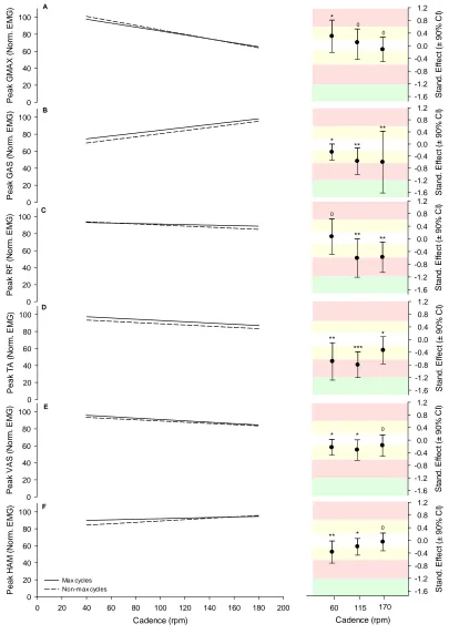
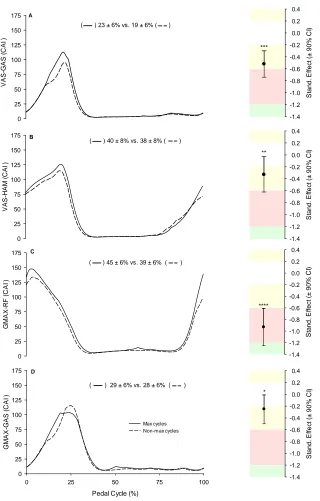
3.3.1 Maximal vs non-maximal pedal cycles ... 65
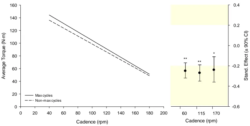
1.1.1.1 Differences in average torque ... 66
1.1.1.2 Differences in peak crank torque ... 66
1.1.1.3 Differences in EMG of the lower limb muscles ... 67
1.1.1.4 Differences in co-activation of the lower limb muscles ... 70
1.1.1.5 Differences in variability of crank torque and EMG profiles ... 71
3.3.2 Prediction of individual T-C and P-C relationships ... 72
3.3.2.1 T-C relationships ... 72
3.3.2.2 P-C relationships ... 75
3.4 Discussion ... 80
xiii
3.4.2 Prediction of T-C and P-C relationships ... 82
3.4.3 Prediction of the limits of lower limb NMF ... 83
3.5 Conclusion ... 85
The Effect of High Resistance and High Velocity Training on a Stationary Cycle Ergometer ... 86
4.1 Introduction ... 86
4.2 Methods ... 89
4.2.1 Participants ... 89
4.2.2 Experimental design ... 89
4.2.3 Training interventions ... 89
4.2.4 Evaluation of RES and VEL training interventions on NMF ... 91
4.2.4.1 Limits of NMF during maximal cycling exercise ... 91
Force-velocity test protocol ... 91
Analysis of T-C and P-C relationships ... 92
4.2.4.2 Control of the pedalling movement ... 92
Crank torque profiles ... 92
Kinematics of the lower limb joints ... 92
EMG activity of the lower limb muscles ... 95
Variability of crank torque, kinematic, EMG and co-activation profiles ... 96
4.2.4.3 Estimation of lower limb volume ... 97
4.2.5 Statistical analyses ... 97
4.3 Results ... 99
4.3.1 Effect of training on lower limb volume ... 99
4.3.2 Effect of training on the limits of NMF ... 99
4.3.2.1 Effect of RES training ... 99
4.3.2.2 Effect of VEL training ... 102
4.3.3 Effect of training on crank torque, kinematic and EMG profiles ... 104
4.3.3.1 Crank torque profiles ... 104
xiv
4.3.3.3 EMG and CAI profiles ... 109
4.3.4 Effect of training on variability of crank torque, kinematic and EMG profiles .. ... 114
4.3.4.1 Inter-cycle variability ... 114
4.3.4.2 Inter-participant variability ... 115
4.4 Discussion ... 117
4.4.1 The effect of RES training on the limits of NMF and associated adaptations .... ... 117
4.4.2 The effect of VEL training on the limits of NMF and associated adaptations .... ... 119
4.4.3 Limitations ... 121
4.5 Conclusion ... 122
The Effect of Ankle Taping on the Limits of Neuromuscular Function on a Stationary Cycle Ergometer ... 124
5.1 Introduction ... 124
5.2 Methods ... 126
5.2.1 Participants ... 126
5.2.2 Experimental design and ankle tape intervention ... 126
5.2.3 Evaluation of the effect of ankle taping on NMF ... 127
5.2.3.1 The limits of NMF during maximal cycling exercise ... 127
Force-velocity test ... 127
Analysis of T-C and P-C relationships ... 128
5.2.3.2 Control of the pedalling movement ... 129
Crank torque profiles ... 129
Kinematics of the lower limb joints ... 129
EMG activity of the lower limb muscles ... 130
Variability of crank torque, kinematic, EMG and co-activation profiles ... 131
5.2.4 Statistical analyses ... 132
5.3 Results ... 133
xv
5.3.1.1 T-C and P-C relationships ... 133
5.3.1.1 Crank torque profiles ... 134
5.3.1 Effect of ankle taping on kinematic and EMG and co-activation profiles .... 136
5.3.1.1 Kinematic profiles ... 136
5.3.1.2 EMG profiles ... 141
5.3.1.1 CAI profiles ... 143
5.3.2 Variability in crank torque, kinematic, EMG and co-activation profiles ... 145
5.3.2.1 Inter-cycle variability ... 145
5.3.2.2 Inter-participant variability ... 146
5.4 Discussion ... 148
5.4.1 Effect of ankle taping on the left side of the P-C relationship ... 148
5.4.2 Effect of ankle taping on the middle of the P-C relationship ... 150
5.4.3 Effect of ankle taping on the right side of the P-C relationship ... 151
5.5 Conclusion ... 152
General Discussion and Conclusions ... 153
6.1 Summary of findings ... 153
6.2 General discussion and research significance ... 154
6.3 Limitations of this research ... 158
6.4 Overall conclusion ... 161
References ... 162
Appendices ... 187
Appendix A: Study one & two participant information documentation ... 187
Appendix B: Study three participant information documentation ... 193
Appendix C: Study one (Chapter 3) participant characteristics ... 199
Appendix D: Study two (Chapter 4) participant characteristics ... 200
Appendix E: Study three (Chapter 5) participant characteristics ... 201
xvi
List of Figures
Figure 2.1. Schematic illustrating the phases of hip, knee and ankle joint movement and the
location of the main muscles involved in the pedalling movement. ... 10
Figure 2.2. EMG profiles of six lower limb muscles during all-out cycling. ... 12
Figure 2.3. Mechanical energy produced by the leg muscles during simulated maximal cycling. ... 13
Figure 2.4. The relationship between pedal cycle duration and cadence. ... 16
Figure 2.5. Force-velocity and power-velocity relationships for a single muscle/joint and for multi-joint movements. ... 19
Figure 2.6. Relationship between tension and sarcomere length of skeletal muscle. ... 20
Figure 2.7. Crank torque profiles. ... 25
Figure 2.8. Schematic representations of muscle synergies identified for maximal cycling. .... 29
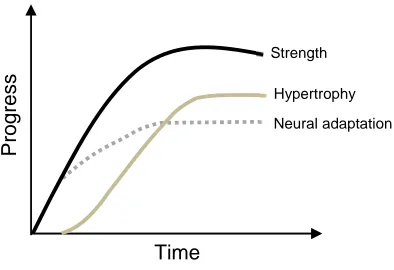
Figure 2.9. Time course for neural and hypertrophy adaptations leading to strength improvements following resistance training. ... 46
Figure 2.10. Work output of muscles during simulated submaximal cycling at 60 rpm. ... 49
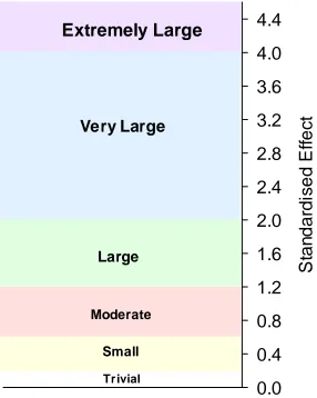
Figure 3.1. Thresholds and associated colour bands used for interpreting the magnitude of the standardised effect ... 64
Figure 3.2. Methods used to select maximal and non-maximal cycles for each participant. ... 65
Figure 3.3. Average torque predicted from maximal and non-maximal cycles ... 66
Figure 3.4. Peak crank torque predicted from maximal and non-maximal cycles ... 67
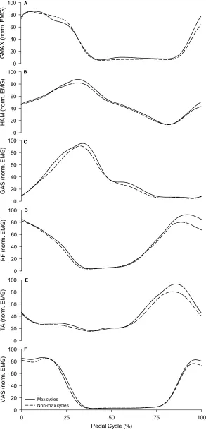
Figure 3.5. EMG profiles from maximal and non-maximal pedal cycles. ... 68
Figure 3.6. Peak EMG predicted from maximal and non-maximal cycles. ... 69
Figure 3.7. Average co-activation profiles and average CAI values for maximal and non-maximal cycles. ... 70
Figure 3.8. Between-cycle VR of EMG profiles and crank torque from maximal and non-maximal cycles. ... 71
Figure 3.9. Goodness of fit variables and residuals estimated from T-C relationships fit with high and low order polynomials. ... 73
xvii
Figure 3.11. Torque predicted from T-C relationships fit with high and low order polynomials
... 74
Figure 3.12. Limits of NMF- T0 and C0 fit with high and low order polynomials. ... 75
Figure 3.13. Goodness of fit variables and residuals estimated from P-C relationships fit with
high and low order polynomials. ... 76
Figure 3.14. P-C relationships fit with high and low order polynomials. ... 77
Figure 3.15. Power predicted from P-C relationships fit with high and low order polynomials 77
Figure 3.16. Limits of NMF- Pmax and Copt fit with high and low order polynomials. ... 78
Figure 3.17. Power predicted from P-C relationships fit with high and low order polynomials at
5 rpm intervals moving away from Copt on the ascending (i.e. negative values) and descending (i.e. positive values) limbs of the relationship. ... 79
Figure 4.1. Sections of the T-C and P-C relationships for which RES and VEL trained during the
four week intervention. ... 91
Figure 4.2. Motion capture marker set up. ... 93
Figure 4.3. Interpretation of hip, knee and ankle joint movement. ... 95
Figure 4.4. Experimental set up for data collection, including the equipment used for mechanical,
kinematic and EMG data acquisition. ... 96
Figure 4.5. Illustration of the sites for anthropometric measurements and the six segments used
to calculate lower limb volume. ... 97
Figure 4.6. P-C and T-C relationships of a single participant before and after RES training. ... 99
Figure 4.7. Power predicted from P-C relationships and torque predicted from T-C relationships
before and after RES training. ... 100
Figure 4.8. Power production at 60-90 rpm and 160-190 rpm before and after RES training. 101
Figure 4.9. P-C and T-C relationships of two participants before and after VEL training. ... 102
Figure 4.10. Power predicted from P-C relationships and torque predicted from T-C relationships
before and after VEL training. ... 103
Figure 4.11. Power production at 60-90 rpm and 160-190 rpm before and after VEL training.
... 104
Figure 4.12. Crank torque profiles before and after RES training at 60-90 rpm. ... 105
xviii
Figure 4.14. Joint angle profiles before and after RES training for 60-90 rpm. ... 107
Figure 4.15. Joint angle profiles before and after VEL training for 160-190 rpm. ... 108
Figure 4.16. EMG profiles before and after RES training at 60-90 rpm. ... 110
Figure 4.17. EMG profiles before and after VEL training at 160-190 rpm. ... 111
Figure 4.18. CAI profiles before and after RES training at 60-90 rpm. ... 112
Figure 4.19. CAI profiles before and after VEL training at 160-190 rpm. ... 113
Figure 5.1. Ankle taping procedure. ... 127
Figure 5.2. Sections of the pedal cycle. ... 129
Figure 5.3. Experimental set up for data collection including the equipment used for the acquisition of mechanical, kinematic and EMG data. ... 131
Figure 5.4. Average power produced during the downstroke and upstroke phases of the pedal cycle in CTRL and TAPE conditions. ... 134
Figure 5.5. Crank torque profiles for CTRL and TAPE conditions. ... 135
Figure 5.6. Ankle ROM for CTRL and TAPE conditions. ... 137
Figure 5.7. Joint angle profiles for CTRL and TAPE conditions. ... 139
Figure 5.8. EMG profiles for CTRL and TAPE conditions. ... 142
xix
List of Tables
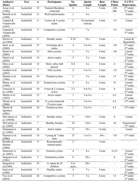
Table 2.1. Summary of studies that have used force-velocity test protocols on stationary cycle
ergometers. ... 42
Table 3.1. Inter-cycle VR for crank torque, EMG and co-activation of muscle pairs from maximal
and non-maximal cycles. ... 72
Table 4.1. Effect of RES training on the limits of NMF estimated from P-C and T-C relationships.
... 101
Table 4.2. Effect of VEL training on the limits of NMF estimated from P-C and T-C relationships.
... 104
Table 4.3. Inter-cycle VR for crank torque, joint angle, EMG and CAI, before and after RES
training at 60-90 rpm. ... 114
Table 4.4. Inter-cycle VR for crank torque, joint angle, EMG and CAI, before and after VEL
training at 160-190 rpm. ... 115
Table 4.5. Inter-participant VR for crank torque, joint angle, EMG and CAI, before and after RES
training at 60-90 rpm. ... 116
Table 4.6. Inter-participant VR for crank torque, joint angle, EMG and CAI, before and after
VEL training at 160-190 rpm. ... 116
Table 5.1. Limits of NMF estimated from P-C and T-C relationships calculated in the downstroke
and upstroke phases of the pedal cycle. ... 133
Table 5.2. Section of the pedal cycle corresponding to the start of joint extension/plantar-flexion
and flexion/dorsi-flexion. ... 136
Table 5.3. Minimum and maximum joint angles and range of motion for the hip, knee and ankle
joints in CTRL and TAPE at 40-60 rpm, 100-120 rpm and 160-180 rpm. ... 138
Table 5.4. Extension/plantar-flexion and flexion/dorsi-flexion velocities for the hip, knee and
ankle joints in CTRL and TAPE at 40-60 rpm, 100-120 rpm and 160-180 rpm. ... 140
Table 5.5. Peak EMG values in CTRL and TAPE conditions at 40-60 rpm, 100-120 rpm and
160-180 rpm. ... 141
Table 5.6. Average CAI values in CTRL and TAPE at 40-60 rpm, 100-120 rpm and 160-180 rpm.
... 143
Table 5.7. Inter-cycle VR for crank torque, kinematic and EMG profiles for CTRL and TAPE
xx
Table 5.8. Inter-cycle VR for crank torque, kinematic and EMG profiles for CTRL and TAPE
conditions at 100-120 rpm... 145
Table 5.9. Inter-cycle VR for crank torque, kinematic and EMG profiles for CTRL and TAPE
conditions at 160-180 rpm... 146
Table 5.10. Inter-participant VR for crank torque, kinematic, EMG and CAI profiles for CTRL
xxi
List of Equations
Eq. 1 Crank power ... 59
Eq. 2 Co-activation index ... 61
Eq. 3 Variance ratio ... 61
xxii
List of Abbreviations
º degrees
º.s-1 degrees per second
π pi
2D two dimensional
3D three dimensional
APF ankle plantar-flexors
ATP adenosine 5’-triphosphate
BDC bottom dead centre
BF biceps femoris
CAI co-activation index
CI confidence interval
CL confidence limit
cm centimetres
Cmax measured maximal cadence
CNS central nervous system
C0 estimated maximal cadence
Copt estimated optimal cadence
CTRL no ankle tape condition
EMD electromechanical delay
EMG electromyography
EXT extension
F force
F0 maximal force
F-V force-velocity
FLX flexion
xxiii
GMAX gluteus maximus
HAM hamstrings
Hz hertz
KEXT knee extensors
KFLX knee flexors
kg kilogram
L litre
LBDC left bottom dead centre
LLV lean leg volume
L-T length-tension
LTDC left-top-dead centre
LGAS lateral gastrocnemius
max maximum
MGAS medial gastrocnemius
min minimum
mm millimetre
ms millisecond
N newton
Nm newton metre
Nm.kg-1 newton metre per kilo of body mass
NMF neuromuscular function
P-C power-cadence
Pmax estimated maximal power
P-V power-velocity
RBDC right bottom dead centre
RER rate of EMG rise
RES high-resistance training
xxiv
RFD rate of force development
RM repetition maximum
RMS root mean square
ROM range of motion
rpm revolutions per minute
RTD rate of torque development
RTDC right-top-dead centre
s seconds
SD standard deviation
SEE standard error of the estimate
SOL soleus
ST semitendinosus
Stand. Effect standardised effect
T0 estimated maximal torque
Topt estimated optimal torque
TA tibalis anterior
TAPE ankle tape condition
T-C torque-cadence
TDC top dead centre
TLV total leg volume
T-V torque-velocity
V0 maximal velocity
Vopt optimal velocity
VAS vastii
VEL high-cadence training
VM vastus medialis
VL vastus lateralis
xxv W watt
W.kg-1 watt per kilo of body mass
xxvi
Preface
Data collection, analysis and interpretations presented in this thesis are my own. Significant contributions include:
In Chapter 3, David Rouffet designed the study; Rhiannon Patten assisted with data collection; Robert Stokes and Rhett Stephen provided assistance with technical design and support; Will Hopkins and Andrew Stewart provided assistance with statistical analysis.
In Chapter 4, David Rouffet and myself designed the study; Simon Taylor provided support with the kinematics component, assisting with data collection and analysis; Rhiannon Patten assisted with data collection and helped supervise training sessions; Robert Stokes and Rhett Stephen provided assistance with technical design and support; Will Hopkins and Andrew Stewart provided assistance with statistical analysis.
1
Introduction
Our ability to successfully execute a functional task requires adequate neuromuscular function (NMF) (i.e. the combined work of the central nervous system and skeletal muscle) to permit the movement. Tasks can range from those performed as part of daily life (e.g. rising from a chair and ascending stairs) to those required in the sporting arena (e.g. jumping, running and cycling) and most often require a large contribution from the lower limb muscles (Dorel et al., 2005; Gardner et al., 2007; Reid et al., 2008; Vandewalle et al., 1987). As such the investigation of NMF is important in research, clinical and sport science settings for a wide range of populations (e.g. healthy individuals, athletes, patients, and the elderly). A range of force-velocity (F-V) tests performed on stationary cycle ergometers have been well used in the literature as the method permits a safe, accurate and reproducible assessment of the capacity of the muscles involved in the movement to generate force and power (Arsac et al., 1996; Dorel et al., 2005; Driss & Vandewalle, 2013; Martin et al., 1997; McCartney et al., 1985; Samozino et al., 2007). Further, due to the design of the stationary cycle ergometer, and the circular trajectory of the pedalling movement, the external resistance and kinematics of the movement can be well controlled making it an ideal exercise to investigate NMF of the lower limbs in different populations. Just as the relationships between force/power vs velocity of single muscle fibers/single muscles have been described previously by muscle physiologists (Hill, 1938; Wilkie, 1950), the data collected from a F-V test on a stationary cycle ergometer can be used to describe the relationships between torque vs cadence and power vs cadence (Arsac et al., 1996; Dorel et al., 2005; Driss et al., 2002; Hautier et al., 1996; Martin et al., 1997; Samozino et al., 2007; Sargeant et al., 1981). Variables commonly calculated from these relationships, such as maximal power, optimal cadence, maximal torque and maximal cadence can then provide an estimate of an individual’s limits of NMF.
2 multi-joint, dynamic movements such as cycling, these physiological, biomechanical and motor control factors have different effects on the level of force that can be produced and transferred by the working muscles to the crank of the cycle ergometer, depending on the level of resistance or velocity at which the movement is performed. Due to the importance of the force and power producing capacity of the lower limb muscles, it is necessary to implement robust methods for their assessment. However, the approached used to obtain experimental data and quantify the limits of NMF using a F-V test on a stationary cycle ergometer are equivocal in the literature (Arsac et al., 1996; Dorel et al., 2005; Martin et al., 1997), as such the most accurate method for its evaluation is unknown and warrants investigation.
Maintaining and improving NMF is necessary for sustaining healthy movement across the lifespan. Accordingly, the improvements of the limits of NMF are a major focus in traditional resistance and ballistic training programs (Cormie et al., 2007; McBride et al., 2002). However, ballistic training is commonly recommended when improvements in power are sought, due to their specificity to many sports, allowing better transfer of adaptations to performance (Cady et al., 1989; Cronin et al., 2001; Kraemer & Newton, 2000; Kyröläinen et al., 2005; Newton et al., 1996). Ballistic sprint training on a stationary cycle ergometer may be effective for improving the limits of NMF as it offers the opportunity to maximally activate muscles over a larger part of the movement, facilitating greater adaptations. Sprint cycling interventions on stationary cycle ergometers have been shown to improve power production within two days to four weeks of training, attributed to motor learning and neural adaptations, although the improvements were not cadence specific (Creer et al., 2004; Martin et al., 2000a). Indeed, the use of exercises performed at high resistances and high velocities have been shown to elicit intervention specific improvements in power in other exercises (Coyle et al., 1981; Kaneko et al., 1983; Lesmes et al., 1978). As such, power training interventions implemented on a stationary cycle ergometer may be useful for improving the limits of lower limb NMF at specific sections of the T-C and P-C relationships, although this is unclear and warrants further investigation.
3 above, the overall goal of this thesis was to better assess, understand and improve the limits of NMF on a stationary cycle ergometer.
Following a review of literature, this thesis is comprised of three chapters outlining the experimental studies undertaken:
I. Chapter 3 (Study one) – Assessing the limits of neuromuscular function on a
stationary cycle ergometer
II. Chapter 4 (Study two) – The effect of high resistance and high velocity training on
a stationary cycle ergometer
III. Chapter 5 (Study three) – The effect of ankle taping on the limits of neuromuscular
function on a stationary cycle ergometer
4
Review of Literature
2.1
Chapter Overview
This review of literature begins with an explanation of the importance of evaluating the limits of NMF or more specifically the ability to produce torque and power in both sport science and clinical settings. Further, this section details the use of stationary cycle ergometers to assess the NMF of the lower limbs. Section two outlines the physiological, biomechanical and motor control factors affecting torque and power production with specific reference to stationary cycle ergometry, while section three delves into methodological considerations for the assessment of the limits of NMF including the type of test protocol and modelling procedures implemented. A fourth section reviews the use of ballistic training interventions to improve NMF and the accompanying neural and morphological adaptations. Lastly, this review documents the role of the ankle joint during ballistic exercises, in particular sprint cycling and the effects of ankle taping on the limits of NMF on a stationary cycle ergometer.
2.2
The importance of understanding, assessing and improving the limits
of NMF of the lower limbs
5
ballistic exercises to assess NMF is emerging in the literature (Hoffrén et al., 2007; Millet & Lepers, 2004; Sarre & Lepers, 2005). With this in mind, in both sport science and clinical settings there is a need to assess NMF using exercises (e.g. cycling) that encompass the muscles largely used in functional tasks.
2.2.1 Limits of lower limb NMF in sport science
The ability to produce a high level of power is considered to be fundamental in a successful sporting performance (Martin et al., 2007; Morin et al., 2002; Vandewalle et al., 1987), with many studies showing that high force and power outputs are well correlated with athletic performance (Baker, 2001; Kraemer & Newton, 2000; Sleivert & Taingahue, 2004). With regards to sprint cycling, a high maximal power output and the ability to maintain a high level of power output over a wide range of cadences is favorable to a successful sporting performance, especially as the velocity of the movement is continually changing over the duration of an event (e.g. a flying 200-m sprint) (Gardner et al., 2007; Martin et al., 2007; Morin et al., 2002; Vandewalle et al., 1987). Indeed, Dorel and colleagues (2005), found that when corrected for frontal area, maximal power was found to be a significant predictor of 200-m sprint performance in their cohort of world class athletes. Similarly, in other ballistic exercises maximal power has been positively correlated with jump height (Vandewalle et al., 1987) and sprint running speed (Morin et al., 2002). Further, during sprint cycling events that require a stationary start (e.g. 1000-m time trial, 500-m time trial, team sprint) a high torque generating capability is required at the start of the event to get the bike into motion as fast as possible, to allow the cyclist to reach velocities that maximise their power output.
6
2.2.2 Limits of lower limb NMF in clinical exercise science
An adequate level of NMF is required by all humans to perform activities of daily living. Muscle power has been strongly linked to the performance of activities of daily living (e.g. sit to stand, climbing stairs), with a reduction in muscle power leading to an inability to perform these activities (Bassey et al., 1992; Clark et al., 2006; Ferretti et al., 1994; Foldvari et al., 2000; Martin et al., 2000c). The maintenance of NMF over the life span improves the ability of an individual to move without assistance which is necessary for maintaining independent functioning and is of great importance to lessen the burden on public health systems. With these findings in mind it appears essential to have testing procedures that can be implemented with older and frail individuals, those recovering from injury and for those with motor impairment disorders (e.g. stroke, cerebral palsy) to monitor their limits of NMF.
Often, lower limb functionality is assessed using single-joint exercises (e.g. knee extension and flexion), evaluating the force and power producing capabilities of a small number of muscles during isometric contractions (Bassey et al., 1992; Clark et al., 2010). However, the results from isometric exercise tests have been previously shown to correlate poorly with dynamic performances (Baker et al., 1994). Although single-joint and isometric exercises are often deemed to be ‘safer’ for clinical populations to perform, they do not appear to provide an ecological evaluation of the power and torque producing capabilities of the lower limb muscles, therefore do not represent the requirements of the tasks and activities performed on a daily basis.
2.2.3 Assessing the limits of lower limb NMF on a stationary cycle ergometer
As maximal cycling is a ballistic, dynamic, multi-joint movement requiring the production of power from the lower limb muscles (the largest muscle mass of the body) it is well suited to provide an overall assessment of NMF. Like other ballistic running and jumping exercises, most of the external force and power is produced by the lower limb muscles during cycling (Nagano et al., 2005; van Ingen Schenau, 1989; Zajac, 2002). Further, as cycling involves repetitive alternating flexion and extension of the lower limb joints and alternating contraction of agonist and antagonist muscles similar to exercises such as running, it is ideal to evaluate the limits of lower limb NMF in a range of different populations and sports.
7
exercise testing laboratories, community gyms and clubs, the ease and affordability of performing a maximal cycling test on an ergometer is high. Furthermore, due to its closed kinetic chain nature and ability for individuals to be seated during the movement it is a relatively safe exercise, with the ergometer modifiable (e.g. upright or dropped hand positioning, flat or clipless pedals, addition of a back rest to improve stability) to suit the population tested (e.g. athletes, elderly, the injured and those with movement disorders) (Janssen & Pringle, 2008). Indeed, several studies have been conducted whereby the stationary cycle ergometer was modified to suit the requirements of the research aim (Lopes et al., 2014; Reiser Ii et al., 2002; Sidhu et al., 2012). Also, unlike other ballistic movements such as jumping and sprint running the risks of falling and injury are very low in stationary cycle ergometry, even for those who are not accustomed to the movement.
2.3
Factors affecting the limits of lower limb NMF on a stationary cycle
ergometer
8
2.3.1 Physiological (neuromuscular) factors
2.3.1.1Activation of the lower limb muscles
Human skeletal muscles function to produce force and motion by acting on the skeletal system causing bones to move about their joint axis of rotation and are primarily responsible for changing posture and locomotion. In order for movement to occur, muscles must produce a contraction that changes the length and shape of the muscle fibers. The activation of motor units is the first event in the sequence of the production of muscle force. The action of a muscle results from the individual or combined actions of motor units which consist of alpha motor neurons and the muscle fibers it innervates. A single muscle is innervated by a motor neuron pool consisting of a collection of alpha motor neurons. These motor neurons are comprised of a cell body, axon and dendrites, enabling transmission of nerve impulses or action potentials from the CNS to the muscle. Along the myelin sheath encased axon, nodes of Ranvier form uninsulated gaps between the myelin sheaths allowing nerve impulses to move toward the terminal branches at the neuromuscular junction. The neuromuscular junction serves as the crossing point between the end of the myelinated motor neuron and a muscle fiber and functions to transmit the nerve impulse to initiate a muscle action. Arrival of an impulse at the neuromuscular junction triggers a release of neurotransmitter acetylcholine, changing the electrical nerve impulse into a chemical stimulus. Within the postsynaptic membrane acetylcholine combines with a transmitter-receptor eliciting a wave of depolarization (action potential) that spreads along the sarcolemma, into the transverse-tubule system for initiation of muscle contraction. Excitation-contraction coupling serves as the mechanism whereby the electrical activity of the action potential initiates chemical events at the cell surface causing muscle contraction, with intracellular calcium ions responsible for regulating cross-bridge cycling and therefore muscle contraction (Klug & Tibbits, 1988).
The active state or level of muscle activation and therefore the amount of force a muscle can exert at a given length and velocity is dependent on the number of motor units recruited by the CNS and the frequency at which action potentials are discharged (Adrian & Bronk, 1929). Motor units are recruited systematically according to size (i.e. Henneman’s size principle), with smaller motor units recruited first, followed by larger motor units, and consequently slow-twitch muscle fibers (type I) recruited before fast-twitch muscle fibers (type II) (Henneman, 1957). The order of which motor units are recruited appears to be the same for isometric and dynamic muscle contractions (Duchateau et al., 2006) and also during more rapid (ballistic) contractions (Desmedt & Godaux, 1978).
9
allowing the extracellular recording of action potentials propagating along the muscle fibers (Merletti et al., 2001). Surface EMG has been used extensively to assess the neuromuscular control of the lower limb muscles during submaximal (Chapman et al., 2009; Chapman et al., 2008a; Chapman et al., 2008b; Chapman et al., 2006; Dorel et al., 2008; Hug, 2011; Hug et al., 2008; Hug et al., 2010) and maximal cycling (Dorel et al., 2012; O'Bryan et al., 2014). The main lower limb muscles involved in the pedalling movement include muscles surrounding the hip, knee and ankle joints. As such, the muscles most commonly assessed using EMG include: gluteus
maximus (GMAX)that functions as a hip extensor; vastus medialis (VM) and vastus lateralis (VL) (when combined are referred to as the vastii (VAS))that function as knee extensors; rectus
femoris (RF) that functions as a hip flexor and knee extensor; semimembranosus(SM) and biceps
femoris (BF)(when combined are referred to as the hamstrings (HAM)) that function as a hip
extensor and knee flexor; gastrocnemius lateralis and gastrocnemius medialis (when combined are referred to as gastrocnemii (GAS)) that function as a knee flexor and ankle plantar-flexor;
10
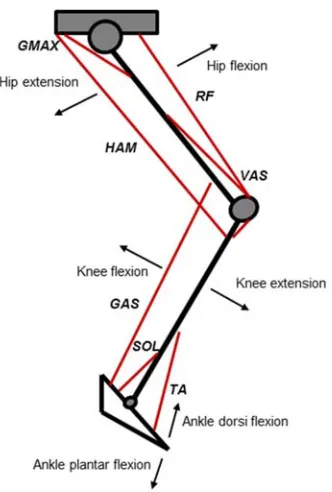
Figure 2.1. Schematic illustrating the phases of hip, knee and ankle joint movement and the location of the main muscles involved in the pedalling movement. GMAX (gluteus maximus), RF (rectus femoris), VAS (vastus lateralis
and vastus medialis), HAM (semimembranosus and biceps femoris), GAS (gastrocnemius), SOL (soleus), TA (tibialis anterior).
Although surface EMG appears to be the most preferred method for assessing muscle active state, physiological (e.g. fiber membrane properties: conduction velocity and synchronisation of motor units, and motor unit properties) and non-physiological (e.g. cross-talk from adjacent muscles, impedance, subcutaneous fat thickness, size and distribution of motor unit territories and electrode placement) factors are known to affect the EMG signal (Farina et al., 2004). Where possible, these factors should be minimised. Accordingly, in an attempt to reduce the effect of electrode placement and standardise the methodology of this technique, recommendations have been produced by the Biomedical and Health and Research Program of the European Union (SENIAM project) (Hermens et al., 2000) and identified in previous research (Rainoldi et al., 2004).
11
signal is typically smoothed using filters (i.e. low-pass, high-pass, band-pass) in accordance with the characteristics of the movement (e.g. the frequency at which its performed) and purpose of EMG analysis in mind. To estimate the level of neural drive to the individual muscles the amplitude of an EMG signal can be assessed. A typical approach taken during voluntary movements to quantify EMG amplitude is the root mean square (RMS) value of the EMG, which reflects the mean power of the signal (Dorel et al., 2008; Laplaud et al., 2006). The timing and duration of muscle activation is also commonly assessed by defining the time of signal burst onset and offset that is often based upon a minimum threshold of three standard deviations of the baseline EMG signal (Neptune et al., 1997; Rouffet et al., 2009). Lastly, the reproducibility of EMG activity levels has been shown to be high during the pedalling movement (Dorel et al., 2008; Houtz & Fischer, 1959; Laplaud et al., 2006).
Due to the aforementioned physiological and non-physiological factors affecting the raw EMG signal, it is difficult to interpret the level of the processed signal without expressing it in relation to a reference value. The EMG signal must be ‘normalised’ to a meaningful and repeatable value, typically a mean or peak EMG to allow comparisons to be made between EMG results obtained from different muscles/subjects or within the same subject on different days. There are several methods which can be used for normalisation including referencing the signal to a peak or mean activation level during isometric and dynamic contractions (Burden, 2010; Burden & Bartlett, 1999; Hug & Dorel, 2009; Rouffet & Hautier, 2008). However, to date there appears to be no consensus as to the most appropriate approach. Using the peak EMG signal from a maximal cycling exercise bout (or more specifically from a F-V test) has been shown to be a valid and reliable way to study muscle activation of the lower limb muscles during cycling (Rouffet & Hautier, 2008). Using this approach the EMG signals of the different muscles recorded during a cycling bout can be expressed as a percentage of the peak muscle activity that occurred during the maximal intensity or reference exercise bout for a given muscle and for a given individual. This normalisation approach has been shown to decrease inter-individual variability in comparison to using a reference value from a maximal voluntary isometric contraction or using the raw EMG data (Chapman et al., 2010; Yang & Winter, 1984). Further, appropriate normalisation lessens the impact of non-physiological factors (e.g. cross-talk, impedance, subcutaneous fat thickness, electrode placement) that can influence the EMG signal (Rouffet & Hautier, 2008).
12
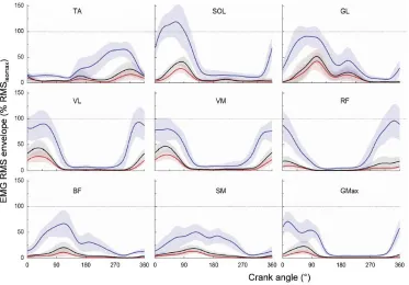
Gregor, 1992). More recently, patterns of lower limb muscle activation during maximal intensity cycling have been illustrated for cadences corresponding to 80% of the participant’s optimal cadence (Dorel et al., 2012). Specifically, as illustrated in
Figure 2.2 below, GMAX was shown to be active during the power producing downstroke
portion of the cycle from 360° (just before top-dead-centre (TDC)) to 120°, while VAS (VL and VM) was also active before TDC at 305° until 100°. RF activity occurred earlier in the cycle (260°) than both GMAX and VAS because of its dual function as a bi-articular muscle and was active to 90°. Medial and lateral GAS appeared to exhibit similar activity patterns, active from TDC, to 220° (beyond bottom-dead-centre (BDC)), while SOL was not active for as long (350° to 140°). Those muscles primarily active during the upstroke (i.e. 180° to 0°) include the HAM group (SM, ST and BF) and TA. HAM was active from 260° to TDC, while TA became active just before BDC up until TDC. It is also important to note that the method for reporting activation patterns can vary between studies, typically for those muscles for which a secondary burst of activation within a pedal cycle can occur (e.g. the bi-articular muscles and TA) (Dorel et al., 2012).
13
Late in the 19th century, the notion that skeletal muscles have different functional roles which are largely dictated by the number (i.e. mono-articular or bi-articular) and type (i.e. ball-and-socket or hinge) of joints the muscle crosses was put forward by Cleland (1867). Since then, it is well accepted that during ballistic exercises such as jumping, sprint running and cycling, mono-articular muscles, those crossing only one joint are suggested to act as primary force producers while bi-articular muscles, those crossing two joints work to transfer the force from the mono-articular muscles and help to control external forces (i.e. the application of force to the crank/pedal in cycling) (Kautz & Neptune, 2002; van Ingen Schenau, 1989; Van Ingen Schenau et al., 1995). Although, it has also been argued that due to the redundant nature of the musculoskeletal system the task being executed will dictate the role a muscle plays regardless of the number of joints it spans (Kuo, 1994).A simulation of maximum speed pedalling has shown that the mono-articular hip (GMAX) and knee extensor (VAS) muscles provide the greatest amount of mechanical energy within a pedal cycle at ~20% and ~35% respectively, while energy produced by the muscles surrounding the ankle (GAS, SOL, TA) and other bi-articular muscles (RF, HAM) are considerably less (Raasch et al., 1997) (Figure 2.3). In agreement, during submaximal cycling Neptune et al. (1997) found that GMAX and VAS produced 80% of their activity during the extension region, while Ericson (1988) reported that muscle force produced during hip and knee extension provided ~70% of total positive work.
Figure 2.3. Mechanical energy produced by the leg muscles during simulated maximal cycling. VAS (vastii), GMAX
14
It appears that maximal muscle activation (i.e. recruitment of all motor units, firing at maximal rates) during a voluntary effort is possible in humans; therefore active state shouldn’t be a limiting factor for the maximal force generating capacity of a given muscle. However, during dynamic movements such as cycling which require the coordination of many muscles, maximal activation would be required by every muscle involved, for every pedal cycle to get a true level of maximal force. Additionally, activation levels are highly variable within and between muscles and individuals, with many repetitions of the movement task often required before a true maximal effort can be generated (Allen et al., 1995). There are a variety of other factors influencing the active state of the muscles involved in the pedalling movement (and subsequently the level of power they can produce) that include movement frequency and subsequent effect on activation-deactivation dynamics; rate of EMG rise; neural inhibitions and post-activation potentiation that are outlined below.
Cadence affects the amount of power (and force) that an individual can produce with increasing cadence imposing two constraints on the neuromuscular system: 1) an increase in joint angular velocity; and 2) decreased time for muscle activation and deactivation (Martin, 2007). Due to the fixed trajectory of the pedal, at a given cadence each muscle will only be active once every pedal cycle, therefore the effect of cadence (or more specifically cycle frequency) on the activity of individual muscles producing the pedalling movement can be easily examined using surface EMG. The effect of cadence on EMG activity level appears to be equivocal, but there is some general agreement that during submaximal cycling, linear increase in GAS, HAM and VAS activity occurred with increasing cadence, while GMAX and SOL exhibited inverted quadratic relationships with the lowest level of EMG occurring at 90 rpm (Ericson, 1986; Neptune et al., 1997). In contrast, reduced VAS and GMAX activity with increasing cadence has been observed by Lucia et al. (2004) in well-trained cyclists. However, less is known regarding the effect of cadence on EMG during maximal effort cycling. Hautier et al. (2000) did not see variations in EMG activity during a 5-s sprint for which cadence reached 150 rpm. Further, Samozino and colleagues (2007) found that average EMG activity did not differ between 70 and 160 rpm for the main muscles involved in the pedalling movement - GMAX, RF, BF, VL.
15
zero)’. During fast cyclical contractions such as pedalling, the effect of activation-deactivation dynamics becomes more influential on the amount of positive and negative work produced by a muscle. The short cycle duration accompanying high cadences starts to become problematic due to the physiological time requirements for the rise and decline of muscle active state and the delay between neural excitation and muscle force response (i.e. electromechanical delay; EMD) (Neptune & Kautz, 2001; van Soest & Casius, 2000). Factors attributed to causing the latency have been suggested to include: the time course of action potential propagation along the sarcolemma into the transverse tubules (i.e. axonal conduction velocity), the processes of excitation-contraction coupling and the time required to stretch the series elastic component of muscle (i.e. force transmission) (Muraoka et al., 2004; Norman & Komi, 1979). However, the contribution of each of these factors to overall EMD is undetermined. EMD has been documented between 30 and 100 ms in duration from onset of muscle active state to peak muscle force (Cavanagh & Komi, 1979; Corser, 1974; Inman et al., 1952; Winters & Stark, 1988) but approximately 90 ms in most of the leg muscles during cycling (Van Ingen Schenau et al., 1995; Vos et al., 1991). It has been suggested that EMD remains relatively constant regardless of movement complexity (Cavanagh & Komi, 1979), cadence (Li & Baum, 2004) and duration for which the movement is performed (Van Ingen Schenau et al., 1992). The functional role of the muscles involved does not appear to affect EMD, with no substantial differences in time reported between mono-articular (93 ± 30 ms) and bi-articular (95 ± 35 ms) muscles (Van Ingen Schenau et al., 1995). As such a blanket EMD of 100 ms has been used in cycling studies when shifting the EMG signal by a given time period or a given portion of the pedal cycle to enable associations to be made between muscle activation and crank torque patterns (Samozino et al., 2007). Using EMG analyses several authors have reported that peak muscle activation occurs earlier in the pedal cycle with increasing cadence, and have suggested that it is a strategy by the CNS to compensate for EMD, in an attempt to maintain a high level of pedal force occurring at the most effective section of the pedal cycle (Neptune et al., 1997; Samozino et al., 2007; Sarre & Lepers, 2007).
16
imposed on the neuromuscular system (Askew & Marsh, 1998). For example at a cadence of 60 rpm each pedal revolution takes ~1-s to complete, with the flexion and extension phases occurring within half that time (~0.5-s) adequate time is available for muscles to reach and maintain a high active state and fully relax within a pedal cycle. As such the effect of activation-deactivation dynamics is minimal at this cadence, with force applied to precise sections of the pedal cycle, which enables power output to be maximised. Alternatively, at higher cadences, such as 180 rpm a pedal revolution takes ~333 ms to complete, with flexion and extension each having to take place within 167 ms. As the physiological time delays for activation and deactivation remain fairly constant, the time required for these processes represent a greater portion of the pedal cycle at higher cadences. Consequently the active state of a muscle is not maximal over the full period for which it shortens and is not zero during the phase at which it lengthens, reducing positive pedal force during the downstroke phase and increasing negative pedal force during the upstroke. Although it should not be forgotten that it is both the combination of muscle active state and increasing shortening velocity contributing to the reduction in pedal force and therefore power with increasing cadence (Martin, 2007; Samozino et al., 2007; van Soest & Casius, 2000).
Figure 2.4. The relationship between pedal cycle duration and cadence.
The speed at which the CNS can maximally activate skeletal muscles at the beginning of a contraction or rate of EMG rise (RER) can also influence the active state of a muscle and corresponding level of power that can be produced. RER is closely linked to the rate of torque development (RTD), the ability to rapidly develop muscular force within the early phase of contraction (Andersen & Aagaard, 2006; Morel et al., 2015). As expected, a high level of
0 200 400 600 800 1000 1200 1400 1600
0 20 40 60 80 100 120 140 160 180 200 220 240 260
Cy
c
le Durat
ion
(m
s
)
Cadence (rpm)
17
contractile RTD is necessary for a good performance in sports requiring high levels of power output, but also for the execution of daily activities and the prevention of injury in the elderly and diseased populations. As outlined above, during ballistic movements such as maximal cycling the time available for muscles to contract can be less than 167 ms (at very fast cadences), though the time required to reach maximal muscular force has been previously shown to be greater than 300 ms in human skeletal muscle (e.g. knee extensors) (Thorstensson et al., 1976b). Consequently, during fast limb movements, the accompanying short period of time available for contraction (e.g. 0-200 ms) may not allow maximal muscle force to be reached and reduce the level of external torque and power produced particularly at high cadences during maximal cycling exercise. RTD has been suggested to be influenced by muscle cross-sectional area, muscle fiber type (i.e. myosin heavy chain composition) and the neural drive to the muscles (i.e. the magnitude of neural drive and rate of motorneuron firing frequency) (Morel et al., 2015).
Acting at the opposite end of the F-V relationship to activation-deactivation dynamics, when the velocity of the movement performed is slow, the level of activation that can be achieved by a muscle or group of muscles can also affected. Previously, it has been shown that during slow knee extension exercises (i.e. when muscle shortening velocity is slow) muscle activation and subsequently torque output were reduced (Babault et al., 2002; Westing et al., 1991). Babault et al. (2002) and Westing et al. (1991) showed that knee extensor muscle activation was reduced concomitantly with slowing muscle shortening velocities (360°.s-1 to 45°.s-1) during concentric maximal knee extension exercise; although the corresponding absolute value of torque was not documented. Further, Caizzo and colleagues (1981) noted that the high force/slow velocity region (~95°.s-1) of the F-V relationship exhibited a levelling off in force output in subjects performing knee extension exercise. It was suggested that the decrease in neural drive reported may be an attempt to limit the generation of high levels of tension in the vastii muscles, a mechanism to protect the musculoskeletal system from injury. More specifically, the Golgi tendon organs sense the high tension levels in the working muscles, increasing inhibitory feedback accordingly to reduce alpha motoneuron excitability and subsequently force output (Solomonow et al., 1988). Although documented in single-joint movements, the occurrence of reduced neural drive in multi-joint movements such as maximal cycling at slow velocities (cadences) is currently unknown.
18
potentiation include an increase in synaptic excitation within the spinal cord, leading to greater post-synaptic potentials and more force produced by the muscles involved (Rassier & Herzog, 2002) and an increased sensitivity of actin-myosin to calcium released from the sarcoplasmic reticulum following subsequent muscle contractions (Grange et al., 1993). It appears that muscle fiber type is the greatest muscle characteristic affecting muscle potentiation magnitude with muscles comprised of a greater proportion of type II fibers exhibiting the greatest potential for muscle potentiation (Hamada et al., 2000). Activities that require short bursts of maximal intensity exercise (such as sprints), adequate recovery between bouts is required to enable phosphocreatine stores to be replenished (McComas, 1996). Although, if recovery is too long the performance enhancing effects of muscle potentiation may be limited due to the lack of preceding muscular contractions before the start of the maximal effort, consequently affecting the level of power produced in the subsequent contractions (i.e. for recurring pedal cycles).
2.3.1.2Muscle force vs velocity and length vs tension relationships
19
fibers. These distinguishing features make these fibers highly resistant to fatigue. Unlike type I fibers, type II fibers can generate energy rapidly, contributing to fast, powerful actions due to speeds of shortening and tension development up to five times higher than type I fibers (Fitts et al., 1989). The characteristics of these muscle fibers include a high capacity for the electromechanical transmission of action potentials, rapid and efficient calcium release and reuptake by the sarcoplasmic reticulum and a high rate of cross-bridge turnover. Type IIb fibers exhibit the fastest shortening speeds of all the fibers, producing very high levels of force, power and speed. Type IIa fibers fall in between type I and type IIb fibers. While still exhibiting a fast shortening speed the capacity for energy transfer is well-developed from both aerobic and anaerobic systems for type IIa fibers making them unable to produce the same level of force as type IIb fibers but more resistant to fatigue. It has been shown that irrespective of conditioning level type IIa fibers can contract 10 times faster than type I fibers and twice as fast as type IIb fibers (Bottinelli et al., 1999; Larsson & Moss, 1993). Further, Sargeant (1994) displayed that the optimal shortening velocity and corresponding maximal power was different between type I and type IIa and IIb fibres.
Figure 2.5. Force-velocity and power-velocity relationships for a single muscle/joint and for multi-joint movements. A: illustrates the force-velocity (black line) and power-velocity (grey line) relationships observed for single muscle and joints, B: illustrates these relationships observed for multi-joint movement. Dotted line denoting the ‘quasi’ linear relationship suggested by Bobbert (2012). Adapted from Hill (1938) and Wilkie (1950).
20
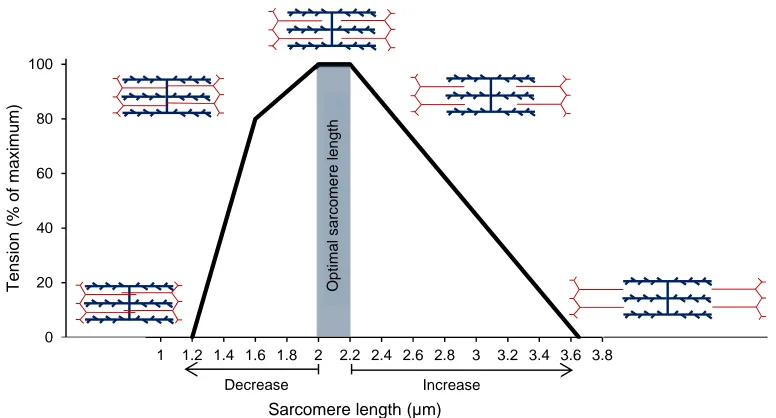
of force only occurs during the attachment phase, the myosin and actin filaments must be close enough to elicit it. As sarcomere length changes, the number of actin binding sites available for cross-bridge cycling changes, with the amount of overlap between the different filaments influencing the amount of the tension that can be generated by the sarcomere. Consequently, a muscle will produce its greatest force when operating close to its ideal length. As illustrated by Figure 2.6, adapted from Gordon and colleagues (1966), when a muscle fiber is shortened or lengthened beyond its ideal length the amount of force the muscle fiber can generate decreases.
Figure 2.6. Relationship between tension and sarcomere length of skeletal muscle. Optimal sarcomere length occurs when the interaction between myosin (blue lines) and actin (red lines) filaments is greatest. Tension output decreases outside of this optimal range as a consequence of too little or too much overlap of the filaments, altering sarcomere length. Adapted from Gordon et al. (1966).
Although it is necessary to understand the mechanics by which a single muscle fiber can produce force, it is the whole muscle comprised of thousands of single muscle fibers and connective tissues positioned about a joint which provides the necessary force for movement. Consequently, the F-V and L-T relationships of whole muscle depends not only on the aforementioned active components of contractile properties (i.e. the active processes of cross-bridge cycling, actin-myosin filament overlap) of the individual muscle fibers but also on passive structures (i.e. Hills three-element muscle model (1938)) which include series (e.g. connective tissues- endomysium, epimysium, perimysium, tendon) and parallel (e.g. the passive force of the connective tissues) and the architecture of the muscle (e.g. fiber type distribution within the muscle, pennation angle
0 20 40 60 80 100
0.4 0.6 0.8 1 1.2 1.4 1.6 1.8 2 2.2 2.4 2.6 2.8 3 3.2 3.4 3.6 3.8
T
ens
ion
(% of
m
a
ximum
)
Sarcomere length (µm)
O
p
tima
l sarcom
ere len
g
th