Impact of Inbound Tourism in Kenyan Economy: An Analysis Using a Computable General Equilibrium Model

IMPACT OF INBOUND TOURISM IN KENYAN ECONOMY: AN ANALYSIS

USING A COMPUTABLE GENERAL EQUILIBRIUM MODEL

Mohamed KARIM

Eric Tchouamou NJOYA

ABSTRACT

In both developing and developed countries tourism is often regarded as an economic activity of immense significance creating thousands of jobs. However, calculations dealing with the economic nature of tourism are often derived from input-output models, which largely overstate its effects on employment by assuming linear responses and highly elastic supplies of goods, services and labor. The purpose of this study is to develop and apply a computable general equilibrium approach to estimate the effects of growth in tourism spending on the Kenyan economy as a whole and on particular sectors within it. The results indicate that the economic benefits from tourism expansion in Kenya are small. The paper concludes with a discussion of the policy implications and research limitations.

Keywords: Tourism sector, Computable general equilibrium model

INTRODUCTION

In the past two decades an increasing number of researchers have sought to determine the impact of

supply and demand shocks in one sector on the economy as a whole. Domestic or international

shocks such as the outbreak of SARS or the terrorist attacks of September 11, 2001 adversely affect

industries such as air transport, tourism and the economy as a whole. This indicates a need to

understand the nature of the impact of shocks and policy changes in order to gain greater insight

into the workings of such changes and determine ways of minimizing their adverse effects.

However, much of the research with reference to developing country up to now has been

descriptive in nature or has relied on input-output (I-O) analysis. The major objective of this study

is to develop and applied Computable general equilibrium (CGE) models to investigate the effects

of a range of alternative policies or exogenous tourist expenditure shocks. Despite the existence of

varied tourist attractions, comprising warm weather, tropical beaches, abundant wildlife in natural

1 _{University of Mohammed V-Souissi, Rabat, Morocco. E-mail:mokarim@voila.fr} 2 _{University of Applied Sciences Bremen. E-mail: Eric.Tchouamou- Njoya@hs-bremen.de}

Asian Journal of Empirical Research

habitats, scenic beauty and a geographically diverse landscape, this potential has in many cases not

been fully exploited. However, in recent years, investment in tourism infrastructure and public

health standards in most developing countries (DCs) has improved. On the other hand, a range of

factors such as higher discretionary incomes, smaller family sizes, changing demographics in many

Northern countries are having a huge impact on tourism demand. Many attempts to explain the

linkages between tourism and economic growth have been made. Development theorists contend

that increased services export (such as tourism) may contribute to economic diversification and to

economic growth.

The net social benefit of tourism growth, that is the reduction of poverty and its effects on income

distribution, is an important and relatively unexplored aspect of tourism in Kenya. Economic

models of research in tourism are dominated by the impact of tourism measured in terms of its

contribution to gross national product, employment and income generation. As a private sector led, outward oriented industry, the question is whether tourism can contribute to Kenya’s urgent need for pro-poor growth - an important area into which this paper will delve. The goal of this paper is to

make use of general equilibrium adjustment mechanisms in answering the following question: will

the expansion of the tourism sector in Kenya advance or retard the broader development goal of

poverty alleviation?

TOURISM AND THE KENYAN ECONOMY

The Kenyan economy has undergone a structural transformation since the country’s independence in 1963. The macroeconomic performance of the Kenyan economy over the years is best

understood in the context of external shocks and internal challenges that the economy has had to

adjust to. There has been a gradual decline of the share of agriculture in overall GDP from 36.6%

in the first decade after independence to about 22.2% in 2011. The share of manufacturing has only

grown slowly and actually accounts for about 16.4% of GDP. The service sector accounts for

64.6% of GDP, with the key sub-sectors being transport and communication, wholesale and retail trade, and hotels and restaurants. Since 2000, Kenya’s GDP growth has improved and remained strong. In 2011, real GDP grew by an estimated 5.7% due to improved performance across all the

key sectors. Inflation has been more volatile, with 2011 inflation measured at 7.2%, up from 3.9%

in 2010. The total population of Kenya was last reported over 40 million in 2010 (according to a

World Bank report released in 2011) from 8.1 million in 1960. The vast majority of people (79% of

total population) lives in rural areas and relies on agriculture for most of its income. The poverty

rate is measured at about 48%.Kenya offers varied tourist attractions, comprising tropical beaches,

abundant wildlife in natural habitats, scenic beauty and a geographically diverse landscape. The

most popular tourist attractions in Kenya are the wildlife and the beaches. According to the World

Travel and Tourism Council (WTTC) (2012), the direct contribution of Travel and Tourism to

to rise by 4.3% in 2012. Travel and Tourism directly supported 313,500 jobs (4.8% of total

employment) and 11.9% at full impact level. A focus on the sub-Saharan country shows that the

travel and tourism sector contributed directly to about 2.6% of total GDP (USD33.5bn) and 2.4%

of total employment (5,265,000 jobs) in 2011. International tourist arrivals generally doubled since

1990 and are still expected to grow steadily at least for the next decade. Most overseas visitors to Kenya come from Europe and America, with Europe accounting for over 70% of the country’s visitors (Ministry of Tourism, 2012).

Tourism is a key part of the country’s economic strategy. Tourism has been recognized as one of the sectors that will drive economic growth towards achievement of Vision 20303. Key drivers in

the tourism sector through which the government aims to achieve Vision 2030 comprise the

following: repositioning of the Coast circuit; opening underutilized parks and providing niche

products. The strategy aims at making Kenya one of the top 10 long haul tourist destinations,

offering diverse and high end experiences by 2012 to a target of five million tourists. The first

National Tourism Policy of Kenya was formulated under Sessional paper No. 8 of 1969, entitled

Tourism Development in Kenya. That policy set growth targets and spelt out strategies on how the government and private sectors would develop tourism so that it becomes one of the Kenyan’s leading economic activities. In 2002, the Ministry of Tourism and Wildlife initiated the process of

developing a comprehensive tourism policy and legislation.

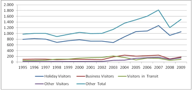
Figure 1: Tourists Arrivals (thousands)

Source: Kenya Tourism Board (http://www.tourism.go.ke/)

It should be noted that package holiday market now dominates demand. The number of tourist

arrivals has increased in recent years as can be seen in Figure-1. Tourism arrivals peaked in 2007,

3_{Kenya Vision 2030 is the country’s new development blueprint covering the period 2008 to 2030. It envisages that Kenya}

but dropped in 2008 to almost 33 % of the 2007 value as a result of post-election violence in

December 2007. Through the 2000s, tourism arrivals grew by an average of 10% per annum.

THE ECONOMIC IMPACT OF TOURISM

Until recently, measurement of the economic impact of tourism has relied on input-output

modeling. Input-output models can be used to assess the value added and inter-industries

relationship attributable to tourism at the country level (Kweka et al. 2003; Archer, 1995; Archer and Fletcher, 1996; Heng and Low, 1990; Seow, 1981 and Khan et al., 1990) and to examine the impact of tourism in a province and city setting (West, 1993; DBEDT, 2002; Frechtling and

Horvath, 1999; Finn and Erdem, 1995). Table-1 reports the multiplier effects of selected applied

I-O studies for developing countries.

Table 1: Selected applied I-O models for developing countries

Economy Authors Main Findings

Egypt Tonamy and

Swinscoe (2000)

Direct tourism jobs constitute 5.7% of national employment – and 12.6% if indirect and induced jobs are included. Tourism contributes over 10% to national GDP

Singapore Heng and Low (1990)

The income impact of one Singapore dollar of tourist expenditure is estimated at S$0.77. Employment multipliers are relatively high (i.e. in 1986, 22 full time equivalent employees per million dollars of tourist expenditure).

Seychelles Archer and Fletcher (1996)

Tourism expenditure Impacts vary by visitor country of origin so that higher spending tourists have a greater economic impact. Tourism contributes approximately 24% to GDP.

However, despite their general equilibrium structure, I-O models do not pay explicit attention to

the effects of tourism on factor incomes or income distribution. Input-output models assume that

wages and prices do not change regardless of the level of production. Thus, I-O analyses do not

take account of resource constraints and crowding out effects. Due to their assumptions, I-O

models may give misleading results. To address this shortcoming, computable general equilibrium

(CGE) models have been widely used in recent years to estimate the economic effects of increases

or decreases in tourism demand (Adams and Parmenter, 1995; Zhou et al., 1997; Dwyer et al.

2000, 2003; Blake et al. 2003a, 2003b, 2006a, 2006b, 2008; Sugiyarto et al. 2003; Narayan, 2004; Madden and Thapa, 2000; Gooroochurn and Milner, 2005; Gooroochurn and Sinclair, 2005;

Kweka, 2004; Polo and Valle, 2007, 2008; Wattanakuljarus and Coxhead, 2008). These models

Table 2: Selected applied Tourism-CGE models for developing countries

Economy Authors Main Findings

Tanzania Kweka (2004)

Tourism has a substantial positive impact on GDP, total welfare, exports and tax revenue. A 20% increase in tourism demand results in an increase in real GDP (at factor cost) of 0.1%. Urban areas will benefit more from tourism expansion than rural areas unless governments invest in improving infrastructure – under this scenario the distributional impact of tourism expansion disproportionally benefits the rural areas.

Indonesia Sugiyarto et al.

(2002)

Tourism growth amplifies the positive impacts of globalization on production and welfare. Globalization, i.e. a 20% reduction in the tariffs on imported commodities combined with a 20% reduction in indirect taxation levied on domestic commodities lead to an increase in demand by foreign tourists by 10%.

Mauritius Gooroochurn and

Milner (2005)

The tourism sectors are undertaxed. Taxing tourism-related sectors would generate an additional unit of tax revenue and increase social welfare in the process. The authors examine the effects of piecemeal, marginal reforms of the indirect taxes (production and sales tax) and, concluding that the additional welfare cost of raising extra revenues from an already existing tax while holding other taxes constant, is lower for sales tax simulations than for the production tax simulations, for all sectors.

Thailand

Wattanakuljarus and Coxhead (2008)

Tourism expansion generates foreign exchange and raises household incomes, but worsens their distribution. Tourism promotion is not a “pro-poor” strategy because tourism sectors are not especially labor-intensive, and their expansion brings about a real appreciation that undermines profitability and reduces employment in tradable sectors, notably agriculture, from which the poor derive a substantial fraction of their income.

Previous applications of CGE modeling to the Kenyan economy were not concerned with tourism.

During the 1980s several authors used CGE models to study the impact of economic reforms on the

distribution of income. The pioneers in this area in Kenya were Dervis et al., (1982) and Gunning (1983). McMahon (1990) examined the effects of unilateral tariff reduction in a dual economy

(Kenya) using a dynamic CGE model on income distribution, concluding that the trickle-down

effects does not take effect since the poorer classes do not consume imported goods or use them in

production.NjugunaKaringi and Siriwardana (2001, 2003) applied CGE modeling to analyze the

effects of macroeconomic stabilization and structural adjustment policies implemented by Kenya in

response to two major terms of trade shocks in the 1970s, namely, the oil price shock and the

coffee export boom. They suggest that fiscal austerity through raising indirect taxes and trade

liberalization supported by foreign aid inflows achieve the best overall outcomes. More recently,

Balistreri et al. (2009) employed a 55 sector small open economy CGE model of the Kenyan economy to assess the impact of services liberalization on both domestic and multinational service

providers. They concluded that reduction of the barriers against potential providers would improve

the productivity of labor and capital and could provide very substantial gains to the Kenyan

MODEL OVERVIEW

The model structure follows closely Robinson et al., (1999). The model builds on that of Dervis et al. (1982), which involve specification of a CGE model in terms of non-linear algebraic equations and addressing them directly with numerical solution techniques. The model is neoclassical in

structure. Its main features involve profit maximization by producers, utility maximization by

households, mobility of labor, and competitive markets. It can be described as a static and

single-country CGE model extended to incorporate international tourism. The model is disaggregated into

two households (urban and rural), two factors (labor and capital), and eight activities and associated

commodities.Cobb-Douglas functions are used for both producer technology and the utility

functions from which household consumption demands are derived (see Appendix B). Exported

and domestically sold commodities are assumed to be differentiated by market, with the

relationship between them represented by a constant elasticity of transformation (CET) function.

Price ratio and elasticities of transformation determined the level of output exported and sold

domestically. Households and producers do not directly consume or use imported commodities but

instead use a so-called “Armington’s composite commodity”, which comprises imports and the

corresponding domestic commodities. The substitution between imports and domestic commodities

is described by a CES function.

Income to enterprises comes from the share of distributed factor incomes accruing to enterprises

and real transfer from the government. Their incomes are used for direct taxes, savings, and

transfers to other institutions. As opposed to households, enterprises do not consume. The

government is disaggregated into a core government account and different tax accounts, one for

each tax type. The government collects taxes and receives transfers from other institutions. The

government uses this income to purchase commodities for its consumption and for transfers to

other institutions as well as savings. The demand for commodities by government for consumption

is defined in terms of fixed proportions. Transfer payments between the rest of the world and

domestic institutions are all fixed in foreign currency.The final institution in the model is the

representative tourist. Total tourism demand for commodities is derived from the assumption that

all tourists are homogeneous, whereby Kenya faces a downward-sloping demand curve for its

tourism exports. There is a representative tourist accounting for the consumption of a certain

quantity of a composite good and service at an aggregated price level (PQc). Analogous to

household demand, tourism demand is obtained by maximizing the utility function of the

representative tourist function to its budget constraint. A Cobb-Douglas demand function is used to

give tourism exports. The demand function can be formulated as follows:

Ytou

tou

PQ

WhereCtouCis the quantity of commodity C consumed by tourist,



in tourism consumption and Ytou the total expenditure (revenue) of inbound tourist, which is

defined as follows:

Vtou

Ytou





.

Where







1

total number of tourist arrival. The household welfare change is captured through the Hicksian

Equivalent Variation (EV), which is one measure of welfare commonly used in the literature. Using

changes in utility level evaluated in monetary terms (i.e. the minimum expenditure level), we

compute the change needed to achieve new equilibrium utilities. The welfare change indicator (EV)

is defined as the amount of money necessary to get the new level of utility. The expression of

equivalent variation is given below:

)

,

(

)

,

(

ep

P

U

ep

P

U

EV





Where the expenditure function

ep

(

P

,

U

)

satisfies the given utility U under the price vector P.

0 0

0 1

h h

h h

h

Y

U

U

U

EV





where 0

h

U , 1

h

U and 0

h

Y are the benchmark utility, the new level utility and the benchmark income

level of household group h, respectively. From the equivalent variation equation, it is clear that

tourism expansion affects household welfare through the effects on prices and consumption.

DATA

The model follows the SAM (Social Accounting Matrix) disaggregation of factors, activities,

commodities and institutions. The database of the model is the Kenyan SAM for 2003, jointly

developed by the Kenya Institute for Public Policy Research and Analysis (KIPPRA) and the

International Food Policy Research Institute (IFPRI). The structure of Kenyan Macro SAM is given

in Table-1.A(see Appendix). The original micro SAM is disaggregated across 50 sectors (22

agriculture, 18 industry and 10 services). However, for this analysis the original SAM has been

adjusted in several ways (i.e. 1 agriculture, 1 manufacture and 6 services). The presence of tourists

in the economy necessitates an additional demand component in the SAM. No detailed

Bank (2010). According to WTTC (2011) foreign visitor exports as a percentage of total exports

accounted for about 17% of total exports. The expenditure categories are quite aggregated and they

are illustrated in Table-3. Besides being much aggregated, the expenditure categories do not

compare exactly with the I-O table of the sectors classification and consequently some amendment is needed. “Accommodation”, “inland transport” and “excursions and park fees” are quite straightforward and are allocated to the hotel and restaurants, transport and communication and the

other services sector respectively. “Food and beverage”, “out-of-pocket expenditure” and “miscellaneous” are quite problematic. The latter is so because it is undefined. “Food and beverages” can actually remain in hotels and restaurants, other manufacturing or in wholesale and retail trade. Part of “out-of-pocket expenditure” will go to the wholesale and retail trade sector but the rest can go to any other sectors. “Food and beverage” is thus allocated to wholesale and retail trade and other manufacturing.

Table 3: Expenditures of inbound tourists in Kenya, 2007

Expenditure Categories

Wildlife Safari Premium Wildlife

Safari Beach (All Inclusive)

$/day % of Total $/day % of Total $/day % of Total

Accommodation 33,35 18,1 168,3 46,6 36,85 20,3

Food/beverage 36,65 19,9 83,44 23,1 18,81 10,4

Excursions and park fees 40,71 22,1 22,98 6,4 5 2,8

Inland transport 50,36 27,4 51,62 14,3 13,35 7,4

Out-of-pocket expenditure 16 8,7 35 9,7 41,43 22,9

Miscellaneous 6,84 3,70 0,00 0,00 65,83 36,30

Total expenditure/bed

night 183,91 100 361,35 100 181,27 100

Average length of stay

(nights) 3 7 7-9

Source: World Bank (2010)

Five sectors are identified as related to tourism as follows: Hotel and restaurant (44%), transport

and communication (2%), retail and wholesale trade (2%), manufacturing (0.2%), and other

services (1%). Their ratio, measured as the proportion of inbound tourism demand out of the total,

is given in brackets. These calculations are based on statistics provided by the Kenya National

Bureau of Statistics4, which estimates tourism revenues at 2% of GDP at market prices for the year

2003 (KSH25.8bn). According to World Bank (2010) studies, the total in-country expenditure of,

for example beach package in Kenya represents 51.7% of total expenditure; 36.7% of which

constitute public sector charges.

SIMULATION RESULTS

We simulate a 10% increase in tourism demand by foreign tourist. The simulation quantifies

changes in production in all industries, changes in employment, earnings, prices and all other

variables in the model. Sectors of the economy that are closely related to tourism would increase

output as the result of the increase in expenditure but there would be some contraction of other

sectors. Table-4 shows the macroeconomic effects of a 10% increase in all tourism demand. A 10%

increase in tourism demand is shown to increase GDP by KSH117,713 million. The GDP increase

is equivalent to 0.12% of GDP. In addition to increasing GDP, the increase in tourism demand is

shown to increase government revenues by 50 million KSH. There is a 0.027 % appreciation of the

real exchange rate, and slight increases in labor demand. An economic rationale for promoting

tourism by developing countries is the improvement of the trade balance by increasing export

earnings. The simulated 10% increase in tourist expenditure results in an increase in total exports

(0.008%) which outweighs the increase in total import (0.001%), resulting in an improvement in

balance payment.

Table 4: Macroeconomic effects of simulations

Effects of additional tourism growth

Base year

value Value

Percentage change

GDP at market prices (from spending side)

(Millions KSH) 949418.343 1067131.343 0.124

Private Consumption (Millions KSH) _{632831.000 748840.000 0.24}

Investment (Millions KSH) _{172670 172728.000 0.00}

Government Consumption (Millions KSH) _{234990.000 235030.000 0.00}

Total Export (Millions KSH) _{235449.000 237322.000 0.08}

Total Import (Millions KSH) _{-342006.000 -342273.000 0.01}

Domestic Output (Millions KSH) _{2002514.320 2002179.74 0.26}

Labor Demand (Millions KSH) _{456820.792 457265.691 0.47}

Exchange Rate (Index) _{1.000 0.973 -0.27}

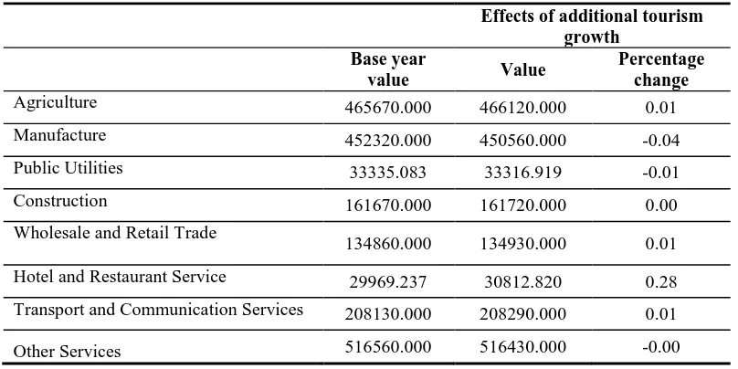
The expansion of tourism is projected to have implications on other industries. Table-5 contains

output projections for 8 sectors aggregated from the 50 sectors distinguished in the 2003 Kenyan

SAM database. The results demonstrate that, at the sectoral level, there will be losers as well as

gainers from an expansion in inbound tourism. The industry level expansion patterns in Table-5

show the largest expansion in the sector that sells a larger proportion of their output to foreign

sector. Particularly poor growth prospects are projected for the construction sector and other

services.

Table 5: Sectoral effects of simulations - Domestic output (Millions KSH)

Effects of additional tourism growth

Base year

value Value

Percentage change

Agriculture _{465670.000 466120.000 0.01}

Manufacture _{452320.000 450560.000 -0.04}

Public Utilities _{33335.083 33316.919 -0.01}

Construction _{161670.000 161720.000 0.00}

Wholesale and Retail Trade

134860.000 134930.000 0.01

Hotel and Restaurant Service _{29969.237 30812.820 0.28}

Transport and Communication Services _{208130.000 208290.000 0.01}

Other Services 516560.000 516430.000 -0.00

Table-6 shows the effects that tourism demand shock has on labor demand. The results indicate that

the effects of increasing inbound tourism on employment closely match with the effects on

domestic output. That is, the industries with large domestic output effects will generate large labor

demand effects. In the simulation results of this study, the largest effects are on the restaurant and

hotel services sector. Effects on the restaurant and hotel services sector trigger an increase in

domestic output of about 0.03% and an increase in the labor demand of about 0.05%.

Table 6: Sectoral effects of simulations - Labor demand

Effects of additional tourism growth

Base year

value Value

Percentage change

Agriculture _{172310.000 172910.000 0.03}

Manufacture _{44903.761 44463.299 -0.10}

Public Utilities _{7972.973 7960.104 -0.02}

Construction _{9167.519 9183.153 0.02}

Wholesale and Retail Trade

17334.885 17364.311 0.02

Hotel and Restaurant Services _{5275.675 5539.298 0.50}

Transport and Communication Services _{41925.979 41995.526 0.02}

As expected, a 10% increase in tourist expenditure impacts on welfare and domestic consumption

output. The simulated positive tourism shock results in a 0.3% increase in rural household

consumption and in a 0.02% increase in welfare (Table-7). Urban household’s consumption and

welfare on the contrary drop by 0.05% and 0.06 respectively. Private consumption increases by

0.18%. Yet the rural household groups are the main beneficiaries of an international tourism

increase. As can be seen from Table-6, a 10% increase in tourism results in an increase in the

domestic consumption of agricultural commodities (0.285%), a decrease in the domestic

consumption of manufacture and service products of 0.005% and 0.03% respectively. From the

previous, it can be concluded that tourism growth in Kenya is pro-agriculture.

Table 7: Results in % change in welfare and household consumption

Economic indicator Percentage change from benchmark

Welfare (EV)

- Rural Household - Urban Household - Net effect

0.02 -0.06 -0.04

Consumption

- Rural Household

o Agriculture

o Manufacture

o Public Utilities

o Wholesale and Retail Trade

o Hotel and Restaurant Service

o Transport and Communication Services

o Other Services - Urban Household

o Agriculture

o Manufacture

o Public Utilities

o Wholesale and Retail Trade

o Hotel and Restaurant Service

o Transport and Communication Services

o Other Services

0.3

o 0.29

o 0.001

o 0.002

o 0.002

o -0.001

o 0.001

o 0.002 -0.05

o -0.005

o -0.006

o -0.004

o -0.006

o -0.02

o -0.006

o -0.005

Price effects are of particular interest in the CGE model. The 10% increase in foreign demand leads

to increases in prices, on average, just under 0.2%, which reduces the growth in tourism

consumption to around 0.04%. Increasing economic activity created by tourism expansion

SENSITITY ANALYSIS

The elasticity parameters for this study have been obtained from existing studies on Kenya, values

assumed in CGE models for other developing countries and guesstimates. Considering the

uncertainties associated with the elasticity parameter of Kenya, sensitivity analysis is used to

demonstrate the robustness of simulation results by varying parameters that may significantly affect

the results. By increasing or decreasing the value of the Armington constant elasticity of

substitution (CES) and constant elasticity of transformation (CET), we examine the range over

which output changes. We define a higher-elasticity case with 20% higher values and a

lower-elasticity case with 20% lower value for those parameters. To evaluate the robustness of the

simulation results, we set the following two criteria: (a) whether the signs of the sectoral output

changes are unchanged in all cases and (b) whether the ordering of the output changes among

sectors is maintained in all cases.The results of the sensitivity analysis shown in Table-7 indicate

that the simulation results satisfy criterion (b) but not criterion (a). More precisely, while the output

of manufacture would always be affected in the same direction in the different assumed elasticity

values, the output of agriculture would increase in the base-line and higher-elasticity cases but

would decrease in the lower-elasticity case.

Table 7: Impact of different elasticity values on sectoral output

Output of: Elasticity of substitution/transformation

Baseline case Higher-elasticity case

Lower-elasticity case

Agriculture 0.01 0.02 0.00

Manufacture -0.04 -0.04 -0.03

Public Utilities -0.01 0.00 0.00

Construction 0.00 0.00 0.00

Wholesale and Retail Trade 0.01 0.00 0.00

Hotel and Restaurant Services 0.28 0.32 0.33

Transport and Communication

Services 0.01 0.01 0.00

Other Services -0.00 -0.00 -0.00

Unit: changes from the base run in %

CONCLUING REMARKS AND RECOMMENDATIONS

In this study we have applied the CGE model to examine the implications on shocks in tourism

expenditures on outputs, income distribution and national welfare. In doing so, this study analyses

the supply side of the tourism sector in Kenya and reviews the literature on tourism using I-O and

CGE with a special focus on developing countries. The analysis indicates that Kenya is endowed

with tourism-attraction potentials. To date, most studies of the economic impact of tourism have

relied on input-output analyses. These studies found that tourism expansion has the potential to

employment for the poor or increasing tax collection. However, CGE models are now increasingly

being used in tourism economics analysis and those applied to developing countries found that

tourism expansion may have an economic cost. The CGE models consist of a set of equations that

characterize the production, consumption, trade and government activities of the economy. The

CGE models enjoy an advantage over I-O models in that they take into account the

interrelationships between tourism, other sectors in the economy and consumers, and have the

ability of incorporating endogenous price determination mechanisms.

Using CGE simulations we analyzed the effects of an increase of 10% in foreign tourist arrivals.

The results show that, overall, the effects of tourism expansion are beneficial but entail costs for

other sectors and for the urban households group. The analysis has shown that a small proportion of

the effects of an increase in tourism demand would be accompanied by an increase in prices. Rural

households, which constitute 77.8 % of the total population (2010) of which 49% are considered

poor, will benefit most from tourism growth. Inbound tourism increases the output of agricultural

products, decreases its prices and increases employment. Agriculture is a major sector from which

rural households derive a substantial fraction of their income (36%). Moreover, these groups spend

a large proportion (53%) of their income on agricultural products. These results indicate a strong

linkage between the agriculture industry and the tourism industry. This finding is in agreement with Summary’s (1987) findings which, comparing the Kenyan tourism industry to other sectors of the economy, established that forward linkages were high in agriculture and that the import content of

the tourism industry was low.

One of the more significant findings to emerge from this study is that the net benefit to Kenyan

from additional tourism is ambiguous. These findings seem to be consistent with other researches.

These authors found that in destinations where tourism is relatively less labor intensive than

agriculture and whose tourism products are mainly intensive user of natural environment (e.g.

Mauritius, South Africa and Zimbabwe), inbound tourism growth will lead to an ambiguous net

benefit on national welfare. Of course, African tourism products (large scale resorts, national parks,

safaris, golf tourism, adventure tourism, etc.) are mainly land-intensive. However, some findings of

this study do not support some previous researches which highlighted that the tourism output

expands at the expense of the agricultural output. It is difficult to explain this result, but it might be

related to the highly aggregated nature of the agricultural sector in the model or the choice of

functional forms and parameters.

In terms of policy implications, one the main issues that emerges from these findings is that when

deciding on tourism development strategy, policy makers should give due consideration to the

overall economic development. Moreover, they should paid attention to the whole range of

distortions that affect the ongoing development of the tourism sector. With regard to the question

alleviation, the findings show that unless governments implement complementary strategies aiming

at mitigating the costs of tourism expansion, economic development and poverty alleviation will

not be attained.

This research is part of an ongoing research designed to develop quantitative information on the

contribution of tourism in Kenya using CGE models. More research on this topic needs to be

undertaken before the association between tourism growth and welfare is more clearly understood.

One of the weaknesses of this study is the choice of the functional forms, which assume a

Cobb-Douglas production and utility function. Alternative functional forms such as a CES production

function or a Stone-Geary utility function (generally preferable since it allows for subsistence

consumption expenditures) may be preferred. Another weakness of this study is the high level of

aggregation of data concerning the agriculture and manufacture sectors, the factor markets and

household categories as well as the tourism industry. Detailed data on tourism expenditures are

needed to improve the understanding of the impact of tourism shocks on different sectors and

institutions. Furthermore, the results would be more useful to tourism policy makers if these

parameter values were empirically estimated. This is an important issue for future research.

Acknowledgements

We would like to thank Nobuhiro Hosoe and Manfred Wiebelt for their help in building the model

and Hans Martin Niemeier, Isabella Odhiambo, Ageliki Anagnostou, Faith Miyandazi and for

reading the paper and providing constructive comments.

REFERENCES

Adams, P. D. and B. R. Parmenter (1995). An applied general equilibrium analysis of the economic

effects of tourism in a quite small, quite open economy. Applied Economics, Vol. 27, pp. 985-994.

Archer, B. (1995). Importance of Tourism for the Economy of Bermuda’, Annals of Tourism

Research Vol. 22, pp. 918-930.

Archer, B. H. and J. Fletcher (1996). The Economic Impact of Tourism in the Seychelles. Annals of Tourism Research, Vol. 23, No. 1, pp. 32-47.

Balistreri, E., T. F. Rutherford and D. Tarr (2009). Modeling services liberalization: The case of

Kenya. Economic Modelling, Vol. 26, No. 3, pp. 668–679.

Blake, A., Sinclair M. T. and Sugiyarto (2003a). Quantifying the impact of foot and mouth disease

on tourism and the UK economy. Tourism Economics, Vol. 9, No. 4, pp. 449-465.

Blake, A. and M. T. Sinclair (2003b). Tourism Crisis Management: US Response to September 11.

Blake, A., R. Durbarry, J., L. Eugenio-Martin., N. Gooroochurn, B., Hay, J. and J. Lennon,

(2006a). Integrating forecasting and CGE models: The case of tourism in Scotland. Tourism Management, Vol. 27, pp. 292-305.

Blake, A., J. Gillham and M. T. Sinclair (2006b). CGE tourism analysis and policy modeling. In L.

Dwyer and P. Forsyth (Eds) International Handbook on the Economics of Tourism,

Cheltenham, Edward Elgar Publishing.

Blake, A., J. S. Arbache., M. T. Sinclair and V. Teles (2008). Tourism and Poverty Relief. Annals of Tourism Research, Vol. 35, No. 1, pp. 107-126.

Clemente, P. A and E. Valle (2007). An Assessment of the Weight of Tourism in the Balearic

Islands’, CRE Working Papers (Documents de treballdel CRE), Centre de Recerca

Econòmica (UIB ·"Sa Nostra").

Dbedt(2002)‘The Hawaii Input-Output Study: 1997 Benchmark Report’, Honolulu: Research and

Economic Analysis Division, State of Hawaii.

Dervis K., De Melo, J. and S. Robinson (1982). General equilibrium models for development

policy. Cambridge, MA: Cambridge University Press.

Dwyer, L., P. Forsyth, J. Madden and R. Spurr (2000). Economic Impacts of Inbound Tourism

under Different Assumptions Regarding the Macroeconomy. Current Issues in Tourism, Vol. 3, No. 4, pp. 325-363.

Dwyer, L., P. Forsyth, R. Spurr and T. Ho (2003). Contribution of tourism by origin market to a

state economy: A multi-regional general equilibrium analysis. Tourism Economics, Vol. 9, No. 2, pp. 117–132.

Finn, A. and T. Erdem (1995). The economic impact in the case of West Edmonton Mall. Tourism Management, Vol. 16, No. 5, pp. 367-373.

Frechtling, D. C. and E. Horvath (1999). Estimating the Multiplier Effects of Tourism Expenditures

on a Local Economy through a Regional Input-Output Model. Journal of Travel Research, Vol. 37, pp. 324-332.

Gooroochurn, N. and M. T. Sinclair (2005). Economics of Tourism Taxation: Evidence from

Mauritius. Annals of Tourism Research, Vol. 32, No. 2, pp. 478-498.

Gooroochurn, N. and C. Milner (2005). Assessing Indirect Tax Reform in a Tourism-Dependent

Developing Country. World Development, Vol. 33, No. 7, pp. 1183–1200.

Gunning, W. J. (1983). Income Distribution and Growth: A Simulation Model for Kenya. In D. G.

Greene (principal author), Kenya: Growth and Structural Change, 2 vols. Washington, D. C:

World Bank, pp. 487-621.

Heng, T. M. and L. Low (1990). Economic Impact of Tourism in Singapore. Annals of Tourism Research, Vol. 17, pp. 246-269.

Karingi, S. N. and M. Siriwardana (2001). Structural Adjustment Policies and the Kenyan

Karingi, S. N. and M. Siriwardana (2003). A CGE Model Analysis of Effects of Adjustment to

Terms of Trade Shocks on Agriculture and Income Distribution In Kenya. Journal of Developing Areas, Vol. 37, pp. 87-108.

Khan, H., C. F. Sengand, and W. K. Cheong (1990). Tourism Multiplier Effects on Singapore.

Annals of Tourism Research, Vol. 17, pp. 408-418.

Kweka, J., O. Morrissey and A. Blake (2003). The economic Potential of Tourism is Tanzania.

Journal of International Development, Vol. 15, pp. 335–351

Kweka, J. (2004). Tourism and the Economy of Tanzania: A CGE Analysis. Retrieved March 31,

2012, http://www.csae.ox.ac.uk/conferences/2004-GPRAHDIA/papers/1f-Kweka-

CSAE2004.pdf

McMahon, G. (1990). Tariff policy, income distribution, and long-run structural adjustment in a

dual economy: A numerical analysis. Journal of Public Economics, Vol. 42, No. 1, pp. 105– 123.

Madden, J., and P. Thapa (2000). The Contribution of Tourism to the New South Wales Economy.

Centre for Regional Economic Analysis, University of Tasmania.

Ministry of Tourism (Kenya), (2012). Tourism performance overview. in websites.

Narayan, P. (2004). Economic Impact of Tourism on Fiji's Economy: Empirical Evidence from the

Computable General Equilibrium Model. Tourism Economics, Vol. 10, No. 4, pp. 419-433. Polo, C. and E. Valle (2007). A General Equilibrium Assessment of the Impact of a Fall in Tourism

Under Alternative Closure Rules: the Case of the Balearic Islands. International Regional Science Review, Vol. 31, No. 1, pp. 3-34.

Robinson, S., A. Y. Naude, R. H. Ojeda, J. D. Lewis and S. Devarajan (1999). From stylized

models: Building Multisector CGE Models for Policy Analysis. North American Journal of Economics and Finance, No. 10, pp. 5-38.

Sahli, M. and J. J. Nowak (2007). Does Inbound Tourism Benefit Developing Countries? A Trade

Theoretic Approach. Journal of Travel Research, Vol. 45, pp. 426-434.

Seow, G. (1981). Economic Impact Significance of Tourism in Singapore. Singapore Economic Review, Vol. 26, No. 2, pp. 64-79.

Sugiyarto, G., A. Blake, and, M.T. Sinclair (2002). Tourism and Globalization: Economic Impact

in Indonesia. Annals of Tourism Research, Vol. 30, No. 3, pp. 683-701.

Summary, R. M. (1987). Tourism's contribution to the economy of Kenya. Annals of Tourism Research, Vol. 14, No. 4, pp. 531–540.

Tonamy, S. and A. Swinscoe (2000) ‘The Economic Impact of Tourism in Egypt’, Working Paper

No.40.

West, G. R. (1993) ‘Economic Significance of Tourism in Queensland’, Annals of Tourism

Research, Vol.20,pp.490-504.

Wattanakuljarus, A. and Coxhead, I. (2008). Is tourism-based development good for the poor?: A

World Bank (2010). Kenya’s Tourism: Polishing the Jewel. Retrieved March 31, 2012.

World Tourism Organisation (2001). The Least Developed Countries and International Tourism. in

Tourism in the Least Developed Countries, edited by the World Tourism Organization.

Madrid: World Tourism Organization.

World Travel and Travel Council (2011). Kenya Economic Impact Report. Retrieved March 28,

2012, http://www.wttc.org/site_media/uploads/downloads/kenya2012_2.pdf.

Zhou, D., J. F. Yanagida, U., Chakravorty and L. Ping Sun (1997). Estimating economic impacts

from tourism. Annals of Tourism Research, Vol. 24, No. 1, pp. 76-89.

Appendix A: SAM Kenya

Table A. 1:2003 Kenya Macro Social Accounting Matrix (Millions of Kenyan Shillings)

Appendix B: The equations of the models

Indices

a



c



c





c





c





C





f



Table B. 1:PARAMETERS

a

ad production function efficiency parameter

a

aq shift parameter for composite supply (Armington) function

c

at shift parameter for output transformation (CET) function

cpi consumer price index

cwts_c weight of commodity c in the CPI

ica_ca quantity of c as intermediate input per unit of activity a

inta_a quantity of aggregate intermediate input per activity unit

iva_a quantity of value-added per activity unit

h

mps share of disposable household income to savings

c

pwe export price (foreign currency)

c

pwm import price (foreign currency)

c

qdtst quantity of stock change

C

QG base-year quantity of government demand

qbarinv(C) exogenous (unscaled) investment demand

c

qinv base-year quantity of private investment demand

sE enterprise saving rate

if

shry share for domestic institution iin income of factor f

c

te exporttax rate

c

tm import tariff rate

c

tq rate of sales tax

ii

tr transfer from institution i’to institution i

i

ty rate of nongovernmental institution income tax

Vtou number of tourist

fa

 value-added share for factor f in activity a

ch

 _{share of commodity c in the consumption of household h}

c

tou

 share of commodity c in tourism consumption

q c

 _{share parameter for composite commodity supply (Armington) function}

t c

 _{share parameter for output transformation (CET) function}

ac

q c

 _{Armington function exponent}







1

t c

 _{CET function exponent}





c



1



q c

 _{elasticity of substitution for composite supply (Armington) function}

t c

 _{elasticity of transformation for output transformation (CET) function}

Table B. 2: VARIABLES

Ctou_c inbound tourist's consumption by sector

EG government expenditures

EXR exchange rate (LCU per unit of FCU)

FSAV foreign savings

GSAV government savings

IADJ investment adjustment factor

PA_a activity price

PD_c domestic price of domestic output

PE_c export price (domestic currency)

PM_c import price (domestic currency)

PQ_c composite commodity price

PVA_a value-added price (factor income per unit of activity)

PX_c aggregate producer price for commodity

QA_a quantity (level) of activity

QD_c quantity sold domestically of domestic output

QF_fa quantity demanded of factor f from activity a

QFS_f supply of factor f

QH_ch quantity consumed of commodity c by household h

QINT_ca quantity of commodity c as intermediate input to activity a

QINV_c quantity of investment demand for commodity

QM_c quantity of imports of commodity

QQ_c quantity of goods supplied to domestic market (composite supply)

QX_c aggregated marketed quantity of domestic output of commodity

Walras dummy variable (zero at equilibrium)

WF_f average price of factor f

WFDIST_f wage distortion factor for factor f in activity a

YE enterprise income

YF_if transfer of income to institution I from factor f

YG government revenue

YI_i income of domestic nongovernment institution

Ytou total expenditure of inbound tourist

UU utility (fictitious)

Table B. 3:EQUATIONS

Price Block

Import price PM_c pwm_c(1tm_c)EXR cCM (1)

Export price PE_cpwe_c(1te_c)EXR cCM (2)

Absorption PQ_cQQ_cPD_cQD_cPM_cQM_c





Market output value

c c c c c

c QX PD QD PE QE

PX      cCX (4)

Activity price





 

C c

ac c

a PX

Value-added price



a PA PQ ica

PVA aA (6)

Production and Commodity Block

C-D technology: Activity production function

_

   F f fa a a fa QF ad

QA  aA (7)

Factor demand fa a a fa fa f QF QA PVA WFDIST

WF  



Intermediate demand QINT_caica_caQA_a aA and cC (9)

Output Function a A a ac c QA

QX 





 cC (10)

Composite supply (Armington) function









c q c q c c q c c q c q c

c

QM

QD

QQ







1

1



_

_

_











Import-domestic demand ratio cq

q c q c c c c c PM PD QD QM              1 1 1

c





Composite supply for non-imported outputs imports QQcQDc cCNM ₍₁₃₎

Output transformation (CET) function

CE

c ₍₁₄₎

Export-domestic supply ratio

1 1 1        _ 

 ct

t c t c c c c c PD PE QD QE   

cCE (15)

Output Transformation for nonexported Commodities QX_cQD_c cCNE (16)

Institution Block

Factor income _{fa fa}

A a

f if

if

shry

WF

WFDIST

QF

YF













I

i and fF (17)

Household consumption demand for marketed commodities









ch

c QH mps t YH

PQ   1 1  cCandhH (18)

Investment demand QINV_cIADJqinv_c cC (19)

Government consumption demand QG_c GADJqg_c cC (20)









c t c t c c t c c t c c

c

at

QE

QD

QX





1

1









Government revenue









c cCE

c c c c c c ent gov f gov C c c c c I i row gov i i EXR QE pwe te EXR QM pwm tm tr shry QQ PQ tq tr EXR YI ty

YG , , ,

(21)

Government expenditures





     I i gov i C c c

c QG tr

PQ

EG _, (22)

Tourism demand Ctou_cPQ_ctou_cYtou (23)

Tourist Revenue (expenditure)

Ytou





Vtou

Enterprise revenue cap ent I i i ent shry tr

YE





(25)

Objective function UUsqr





System Constraint Block

Factor market f A a fa QFS QF 



f (27)

Composite commodity markets





c QINT QH QG QINV qdst CTOU

QQ cC (28)

Current account balance for rest of the world (in foreign currency)











c QM tr pwe QE tr PQ EXR Ctou FSAV

pwm _{, ,} / (29)

Savings-Investment Balance





MPS _c

C

c cC

c c c i i I i

i       







 



) (

1 (30)

Price Normalization

