The transformation of gravity waves by
a horizontally sheared current.
Ruairi Donald M aclver
A dissertation subm itted to the U n iversity o f L ond on in partial fu lfilm en t o f the requirem ents for the d egree o f D o c to r o f P h ilo so p h y
D epartm ent o f C ivil and E nvironm ental E ngin eering, U n iversity C o lleg e L ondon
ProQuest Number: 10013943
All rights reserved
INFORMATION TO ALL USERS
The quality of this reproduction is dependent upon the quality of the copy submitted.
In the unlikely event that the author did not send a complete manuscript
and there are missing pages, these will be noted. Also, if material had to be removed,
a note will indicate the deletion.
uest.
ProQuest 10013943
Published by ProQuest LLC(2016). Copyright of the Dissertation is held by the Author.
All rights reserved.
This work is protected against unauthorized copying under Title 17, United States Code.
Microform Edition © ProQuest LLC.
ProQuest LLC
789 East Eisenhower Parkway
P.O. Box 1346
Abstract
The thesis describes a unique experiment conducted in the UK Coastal Research Facility (UKCRF) to
investigate the transformation o f near-hnear gravity waves propagating across a narrow horizontally
sheared jet-like current in constant depth water. The UKCRF is a novel large-scale wave basin
incorporating a multi-directional wave generator and a refined current generation system making it
ideally suited to the study of three-dimensional wave-current interactions. Setting the current
generation system required particular care to create a jet-like current that remained uni-directional and
produced minimal recirculation within the basin. A single wave condition was studied, propagating
across the current orthogonally and at oblique incidence, in both a following and opposing sense to the
current. The length-scale of the current’s shear layers was comparable to the incident wavelength.
The experiment is the first attempt to assess the kinematics and dynamics o f the interaction o f regular
waves and currents in three-dimensions at a physically realistic scale. The resulting benchmark data
set provides direct quantitative measurements of the spatial variation o f the primary flow variables, the
velocity vector, u, and the surface elevation, 77. Observations showed the following wave to be refracted to a more current-parallel direction with an increased wavelength and reduced wave height
as it moved onto the current, while the opposing wave became more current-normal with a shortened
wavelength and enhanced wave height. NegUgible reflection of the incident wave at the current shear
layers was observed.
Four analytical models, each making different assumptions about the current properties, are compared
with the data set to assess their suitability for predicting wave transformation by narrow jet-like
currents. Predictions based on the WKBJ approximation agree well with the trends observed in the
data indicating a slowly-varying current behaviour. The classification o f a current as rapidly- or
Acknowledgements
I am indebted to my supervisor Richard Simons for his patient guidance and encouragement throughout
the course of this research and particularly during the completion o f this dissertation. I would also like
to thank Tony Grass for his helpful comments in my time with the Fluid Mechanics Group.
The research was funded by the Commission of the European Communities Directorate General for
Science, Research and Development under Contract M AS3-CT95-0011 as part o f the Kinematics and
Dynamics of Wave-Current Interactions (KADWCI) project. I appreciated the friendly and supportive
atmosphere that existed between the members of this group, in which fruitful discussions were
conducted with good humour. I would particularly like to thank Gareth Thomas, for assisting my
understanding of theoretical matters, and Maarten Dingemans for drawing my attention to his excellent
book.
I would also like to thank the technical staff of the Department o f Civil & Environmental Engineering
and particularly Bill Fairman and Keith Harvey, of the Fluid Mechanics Group, for their humour and
Table of contents
Abstract 2
Acknowledgements 3
Table of contents 4
List o f figures 7
List o f tables 13
Nomenclature 14
Chapter 1:
Introduction & Literature R eview ... 16
1.1 Introduction 16
1.2 Wave Transformations 17
1.2.1 Surface Waves 18
1.2.2 Currents 19
1.2.3 Current-induced wave transformations 20
1.3 Developments in wave-current transformation modelling 21
1.3.1 Fundamental studies - uniform current 22
1.3.3 Horizontally sheared current 28
1.3.3.1 Slow variation 29
1.3.3.2 Discontinuous variation 35
1.3.3.3 Arbitrary variation 39
1.4 Experimental studies of wave transformation 41
1.4.1 Field studies 41
1.4.2 Laboratory studies 46
1.5 Thesis objectives 51
Chapter 2:
Wave current interaction th eo ry ... 52
2.1 Linear wave solution on homogeneous flow 52
2.2 Linear wave solution on a slowly-varying inhomogeneous flow 55
2.2.1 Slowly-varying flow 55
2.2.2 Slowly-varying flows involving caustics 59
2.2.3 Mild shear approximation 64
2.3 Linear wave solution on a discontinuously-varying inhomogeneous flow 66
2.3.1 Depth independent current 67
2.3.2 Smith’s approximate model 72
2.3.3 Currents with vertical variation 76
2.4 Linear wave solution on an arbitrarily-varying inhomogeneous flow 78
Appendix 2A: Linear wave motion on still water 83
Appendix 2B: Evaluation of the integral term in the Mild Shear Equation. 86
Chapter 3:
Experimental facility, instrumentation and analysis techniques . 93
3.1 The UK Coastal Research Facility 93
3.1.1 Overview 93
3.1.2 Co-ordinate system 95
3.1.3 Wave generation 95
3.1.4 Current generation 98
3.1.5 Instrument bridge 99
3.1.6 Data acquisition system 100
3.1.7 Video 100
3.2 Instrumentation 100
3.2.1 Surface elevation 101
3.2.2 Velocity 103
3.3 Primary data analysis techniques 110
3.4 Secondary data analysis techniques 112
3.4.1 Wave propagation direction 112
3.4.1.1 Velocity vector techniques 112
3.4.1.2 Wave probe array techniques 114
3.4.1.3 Dispersion relation technique 115
Chapter 4: Design of experiments and preliminary t e s t s ... ...118
4.1 Wave properties 119
4.1.1 Oblique wave generation 119
4.1.2 Wave stability 121
4.1.3 Preliminary experiments 122
4.2 Current properties 127
4.2.1 Controlling cross-shore current profiles 128
4.2.2 Current strength 130
4.2.3 Development of a jet current 132
4.3 Proposed measurements 138
4.3.1 Sample durations 139
Appendix 4A: Pump settings and sluice gate apertures 142
Chapter 5:
R esu lts... ...144
5.1 The jet-like current 144
5.1.1 Mean characteristics 144
5.1.2 Temporal variations 153
5.1.3 Theoretical model descriptions of the current 157
5.2 Wave alone conditions 158
5.3 Combined wave and currents 175
5.3.1 Mean current characteristics 175
Chapter 6:
D iscu ssio n ...199
6.1 Model predictions 199
6.1.1 WKBJ Approximation 199
6.1.2 Mild shear equation model 205
6.1.3 Vortex sheet model 206
6.1.4 3D Moderate Current Approximation model 211
6.2 Model performance 212
6.3 Experimental study 215
Chapter 7:
C onclusions... 219
7.1 Conclusions 219
7.2 Future research 221
7.2.1 Recommendations for experimental development 221
7.2.2 Recommendations for model developments 224
References ...225
List of figures
Figure 1.1: Classification o f surface waves (taken from Kinsman ( 1984), figure 1.2-1). 18 Figure 1.2: The nearshore current system: (a) a schematic diagram; (b) field measurements
(taken from Horikawa & Sasaki (1972), figure 1 and figure 12). 20
Figure 1.3 Figure 1.4 Figure 1.5
Definition of wave propagation direction relative to the current direction. 24
Solutions to the Doppler-shifted dispersion relation. 24
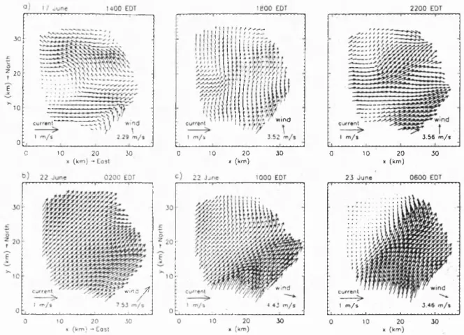
Examples of surface current vectors measured with HF radar: a) tidal flow, b) wind induced flow, and c) Gulf Stream boundary (taken from Shen et al. (2000),
figure 3). 43
Figure 1.6: The experimental facility for Hughes & Stewart’s (1961) study o f wave transformation by a horizontally sheared current (taken from Hughes & Stewart
(1961), figure 1). 46
Figure 1.7: The experimental facility for Hales & Herbich’s (1972) study o f wave transformation by jet-like ebb-flows from a tidal inlet (taken from Hales & Herbich
(1972), figure 1). 47
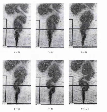
Figure 1.8: Streak photograph indicating the structure o f the ebb flow from a tidal inlet in
the absence o f waves (taken from Hales & Herbich (1972), figure 7). 48
Figure 1.9: Qualitative example of the transformation o f a gravity wave normally incident upon a jet-like ebb flow from a tidal inlet. Waves are propagating from left to right towards the inlet mouth located centre right. Incident wave length decreases from
upper to lower photograph (taken from Hales & Herbich (1972), figures 11-13). 49 Figure 1.10: Time-lapse streak photography of a jet-like current emerging into a still basin.
The merging of turbulent eddies (separately numbered in the first image) can be observed through the sequence. Water depth is four times greater than inlet width
(taken from Dracos et al. (1992), figure 12). 50
Figure 2.1: Coordinate system. 53
Figure 2.2: W ave refraction across a slowly-varying shear layer (adapted from Jonsson
(1990), figure 10). 56
Figure 2.3: W ave ray behaviour on a jet-like current. Upper image - total reflection at caustic line. Lower image - partial reflection at a near-caustic line (adapted from
Peregrine (1976), figure 9). 58
Figure 2.4: Coordinate system and current profile for slowly-varying jet-hke current
IZ=(f/(y,z),0,0). 59
Figure 2.5 : Coordinate system and current profile for vortex sheet representation o f a jet-like
current. 67
Figure 3.1 Figure 3.2 Figure 3.3
Schematic o f the UK Coastal Research Facility. 94
The wave generation system of the UK Coastal Research Facility 95
Oblique wave generation in a basin with fixed internal boundaries, (a) Difficulties: (1) diffraction; (2) reflection at boundaries; (3) local disturbances at
wave generator, (b) Effect o f preventative measures. 97
Figure 3.4: The wave probe array (after Teisson & Benoit, 1994). 101
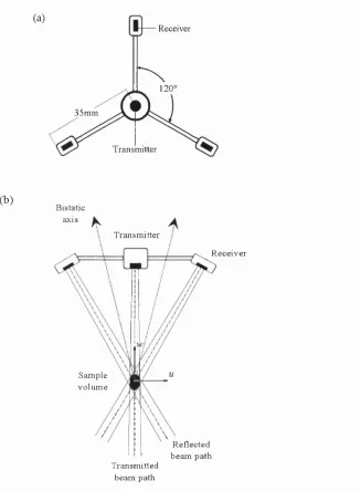
Figure 3.6: The acoustic Doppler velocimeter (ADV) probe: (a) plan, (b) elevation, in
which the third receiver has been omitted for clarity. 105
Figure 3.7: Schematic of the ADV system as deployed in the UKCRF. Components: (a) the
ADV system; (b) transmission line; (c) the data acquisition system. 107
Figure 3.8: Arrangement of the ADV probes and their relation to the basin coordinates: (a) arrangement A, tests involving the jet current alone and the oblique incidence waves;
(b) arrangement B, tests involving the normal incidence wave. 108
Figure 3.9: Recovering the wave propagation direction from the measured horizontal velocity vector: (a) theoretical velocity vector for long crested waves; (b) measured
velocity vector; (c) first harmonic velocity vector. 113
Figure 3.10: Recovering the wave propagation direction from surface elevation
measurements. 115
Figure 3.11: Sketch for recovery of incident and reflected wave parameters (adapted from
Isaacson (1991), figure 2). 116
Figure 4.1: W ave ray theory prediction of refraction for waves at oblique incidence to a following and an opposing current. Incidence angle measured relative to current
normal. 119
Figure 4.2: Paddle element positions during the generation o f an oblique incidence wave. 120 Figure 4.3: Relative amplitudes of the required (p=0) and the first four spurious (p = ± l, ±2)
wave modes when generating an oblique wave (taken from Schaffer (1998), figure
3). 120
Figure 4.4: The range of validity of several common wave theories (taken from Le Méhauté
(1976), figure 7). 122
Figure 4.5: The influence of the wave generation active absorption system on the quality o f
the wave train: (a) without active absorption; (b) with active absorption. 124 Figure 4.6: The influence of the method of determining the underlying oscillatory period in
calculating ensemble average properties. Three different methods have been used: a zero crossing period of surface elevation time series; a zero crossing period of reference signal time series; a specified repeat period. The zero crossing wave height is 0.0325m with zero crossing crest and trough elevations indicated by the horizontal
dashed lines. 125
Figure 4.7: The ensemble averaged surface elevation profile together with the first three harmonic components thereof: (a) normal incidence wave (90°); (b) oblique incidence
wave (60°). A second order Stokes surface elevation profile is also shown 126 Figure 4.8: The stages of development of a plane turbulent jet (taken from Tennekes &
Lumley (1976), figure 4.7). 128
Figure 4.9: Flow past a drowned sluice gate. 129
Figure 4.10: The cross-shore profile of the jet-like current. 131
Figure 4.11: Flow patterns observed in the UKCRF at various stages o f the development o f
the jet-like current. 134
Figure 4.12: Development of the jet-like current across the measurement section (phase 1). Depth averaged horizontal velocity components at three shore-normal sections: o , 5m upstream of basin centre-line; •, basin centre-line; a , 5m downstream o f basin
centre-line. 135
Figure 4.14: The cross-shore profile of the jet-hke current (phase 2). o , depth averaged horizontal velocity components on the basin centre-line. •, repeated measurements
with slight adjustment to inlet sluice gate apertures. 137
Figure 4.15: Typical temporal variation of the jet-hke current velocity components: u,
stream-wise; v, span-wise; w, vertical. Measurements made near the current
centre-hne. 139
Figure 4.16: Variation o f mean velocity with sample length. 140
Figure 4.17: Variation o f the ensemble averaged wave height with number o f wave cycles
included in the calculation. 140
Figure 5.1: Vertical profiles o f the mean stream-wise velocity at locations across the jet current. Error bars indicate the standard deviation o f the velocity. The dashed hnes are to indicate individual profiles and do not represent velocity away from the
measurement locations. 145
Figure 5.2: Span-wise profiles of mean stream-wise velocity at several elevations. The sohd line represents a least squares fit of the Gaussian distribution, equation [5.1] for each profile. The error bars indicate the standard deviation o f the velocity, (a) Elevation 1: ADV2, A D V l, ADVO at z=360,2 0 0 ,40mmrespectively; (b) Elevation 2: ADV2, A D V l, ADVO at z=400, 240, 80mm respectively; (c) Elevation 3: ADV2, A D V l, ADVO at z= 4 40 ,2 8 0 ,120mmrespectively; (d) Elevation 4: A D V l, ADVO at z=320,
160mm respectively. 147
Figure 5.3: Power Law representation of the vertical distribution o f the mean stream-wise
velocity at locations across the jet current. Variable power law exponent. 148 Figure 5.4: Power Law representation of the vertical distribution o f the scaled mean
stream-wise velocity. Constant power law exponent. 149
Figure 5.5: Span-wise variation of depth-averaged approximations o f the mean stream-wise
velocity. 151
Figure 5.6: Development of the depth-averaged jet current velocity through the test region. Solid lines are least squares regressions o f the Gaussian-like profile, equation [5.1],
dashed lines are least squares regressions o f the sech^ profile, equation [5.2]. 152 Figure 5.7: Time series and low frequency detail o f the energy density spectrum o f the
orthogonal velocity components measured near the centre-line o f the mean jet current, y=6.386m. Measurements made at approximately mid-depth, z=240mm. Frequency
resolution o f spectra 0.005Hz. 154
Figure 5.8: Time series and low frequency detail o f the energy density spectrum o f the orthogonal velocity components measured near the off-shore edge o f the mean jet current, y=3.386m. Measurements made at approximately mid-depth, z=240mm.
Frequency resolution o f spectra 0.005Hz. 155
Figure 5.9: Full range energy density spectrum of the orthogonal velocity components: (a) near the mean current centre-line; (b) near the off-shore edge o f the mean current. Measurements made at approximately mid-depth, z=240mm. Frequency resolution
o f spectrum O.lHz. 156
Figure 5.10: Surface elevation time series at locations across the basin centre-line for a wave
in the absence of the jet current, (a) y=3.4m, (b) 5.4m, (c) 7.4m, (d) 9.4m. 159 Figure 5.11: Variation of the 1st harmonic wave height for normal incidence waves in the
absence of the jet current (WAN). Solid line is a prediction o f the modulation caused
Figure 5.12: Variation of the 1st harmonie wave height for oblique incidence wave in the absence of the jet current (WAF). Solid line is a prediction of the modulation caused
by spurious waves. 161
Figure 5.13: Variation of the 1st harmonic wave height for oblique incidence wave in the absence of the jet current (WAO). Solid line is a prediction o f the modulation caused
by spurious waves. 161
Figure 5.14: W ave propagation directions inferred from the surface elevation phase differences between all eight probes of the wave probe array. Nominal propagation
directions: WAF condition, 60°; W AN condition, 90°; W AO condition, 120°. 163 Figure 5.15: Phase speed inferred from the surface elevation phase differences between all
eight probes o f the wave probe array. The dashed line indicates the global estimate
o f the phase speed. 163
Figure 5.16: The span-wise variation in horizontal velocity components for an oblique incidence wave in the absence of the jet current (WAF). Upper part: oscillatory components, ensemble averaged vector (solid line), first harmonic vector (dashed
line). Lower part: mean components. Measurements at z=310mm by A D V l. 165 Figure 5.17: The span-wise variation in horizontal velocity components for an oblique
incidence wave in the absence of the jet current (WAO). Upper part: oscillatory components, ensemble averaged vector (solid line), first harmonic vector (dashed
line). Lower part: mean components. Measurements at z=310mm by A D V l. 166 Figure 5.18: The span-wise variation in wave propagation direction, estimated from the
horizontal velocity vector at several vertical elevations, for an oblique incidence wave
in the absence o f the jet current (WAF). 168
Figure 5.19: The span-wise variation in wave propagation direction, estimated from the horizontal velocity vector at several vertical elevations, for an oblique incidence wave
in the absence o f the jet current (WAO). 169
Figure 5.20: The span-wise variation in wave propagation direction, estimated from the horizontal velocity vector at several vertical elevations, for normal incidence wave
in the absence o f the jet current (WAN). 170
Figure 5.21 : Comparison of wave propagation direction inferred from the measured velocity vector and a prediction based on the velocity vector produced by the wave components identified as producing the wave height modulation: (a) WAF case (b)
WAO case (c) W AN case. 171
Figure 5.22: Vertical variation of the first harmonic amplitude o f the horizontal velocity vector at several locations across the basin centre-line (WAF case). Solid line
indicates the linear wave theory prediction for finite depth water. 173
Figure 5.23: Vertical variation of the first harmonic amplitude o f the vertical velocity at several locations across the basin centre-line (WAF case). Solid line indicates the
linear wave theory prediction for finite depth water. 174
Figure 5.24: Vertical profiles of the mean stream-wise velocity at locations across the jet current under combined wave-current conditions. Normal incidence wave (WCN). The dashed lines are to indicate individual profiles and do not represent velocity away
from the measurement locations. 176
Figure 5.25: Vertical profiles of the mean stream-wise velocity at locations across the jet current under combined wave-current conditions. Following oblique wave (WCF). The dashed lines are to indicate individual profiles and do not represent velocity away
Figure 5.26: Vertical profiles o f the mean stream-wise velocity at locations across the jet current under combined wave-current conditions. Opposing oblique wave (WCO). The dashed lines are to indicate individual profiles and do not represent velocity away
from the measurement locations. 178
Figure 5.27: Vertical profiles of stream-wise velocity at current centre-line for the JET condition and all combined conditions. The dashed lines are to indicate individual
profiles and do not represent velocity away from the measurement locations. 179 Figure 5.28: Jet current velocity distribution on basin centre-line for the combined
wave-current tests. 180
Figure 5.29: Variation of wave phase along the measurement section for the oblique incidence combined wave-current conditions. The variation for the oblique wave alone condition is shown for comparison. The wave phase is shown relative to that o f the
first measurement point. 181
Figure 5.30: Variation in wave phase along the measurement section for a normal incidence wave both in the presence of, and also the absence of, the jet current. Phases are
relative to that o f the first measurement point. 182
Figure 5.31 : Surface elevation time series at locations across the measurement section for the
combined wave-current case WCF. (a) y=3.4m, (b) 5.4m, (c) 7.4m, (d) 9.4m. 183 Figure 5.32: The influence of the current on the mean and standard deviation o f the zero
crossing wave period, (a) Measurements o f mobile wave probe 1 at locations across the basin centre-line, (b) Measurements of static wave probe A during the traverse
across the basin centre-line 184
Figure 5.33: Surface elevation spectra of waves in the absence o f the jet current. Spectra are
of the time series presented in figure 5.10, with a frequency resolution o f 0. IHz. 185 Figure 5.34: Surface elevation spectra of waves in the presence o f the jet current. Spectra are
of the time series presented in figure 5.31, with a frequency resolution o f O.lHz. 185 Figure 5.35: Variation of wave height for normal incidence combined wave-current condition
(WCN). 186
Figure 5.36: Variation of wave height for the oblique incidence combined wave-current
condition WCF. 187
Figure 5.37: Variation of wave height for the oblique incidence combined wave-current
condition WCO. 187
Figure 5.38: Variation in the wave propagation direction, a, established from the surface elevation phase lags, for the three combined wave-current conditions: (a) WCF, (b) WCO, (c) WCN. The dashed lined indicates the direction o f the wave alone
conditions. 189
Figure 5.39: Variation in the wave propagation direction, a, established from the oscillatory
velocity vectors for the combined wave-current condition WCF. 190
Figure 5.40: Variation in the wave propagation direction, a, established from the oscillatory
velocity vectors for the combined wave-current condition WCO. 191
Figure 5.41: Variation in the wave propagation direction, a, established from the oscillatory
velocity vectors for the combined wave-current condition WCN. 192
Figure 5.42: Comparison of the wave propagation direction, a, established from the surface elevation phase lag and the oscillatory velocity vector for each of the combined
Figure 5.43: Least squares optimisation of equation [5.10] to the wave phase variation for the
oblique incidence combined wave-current conditions. 194
Figure 5.44: Variation in the wave phase velocity, established from the surface elevation phase lag, for the three combined wave-current conditions: (a) WCF, (b) WCO, (c)
WCN. 196
Figure 5.45: The span-wise variation in horizontal velocity components for the oblique incidence combined wave-current condition WCF. Upper part: oscillatory components, ensemble averaged vector (solid line), first harmonic vector (dashed line) and the principle wave direction (straight line). Lower part: mean components.
Measurements made at z= 310mm by instrument A D V 1. 197
Figure 5.46: The span-wise variation in horizontal velocity components for the oblique incidence combined wave-current condition WCO. Upper part: oscillatory components, ensemble averaged vector (solid line), first harmonic vector (dashed Une) and the principle wave direction (straight hne). Lower part: mean components.
Measurements made at z= 310mm by instrument ADV 1. 198
Figure 6.1: WKBJ prediction o f the variation of wave properties for the combined wave-current condition, WCF: (a) phase velocity; (b) propagation direction (established from the wave probe array); (c) wave height. Incident wave height taken to be
0.032m. 201
Figure 6.2: WKBJ prediction o f the vertical velocity amphtude for the combined
wave-current condition WCF. Comparison to measured amplitudes. 202
Figure 6.3: WKBJ prediction o f the variation o f wave properties for the combined wave-current condition, WCO: (a) phase velocity; (b) propagation direction (established from the wave probe array); (c) wave height. Incident wave height taken to be
0.032m. 203
Figure 6.4: WKBJ prediction of the vertical velocity amplitude for the combined
wave-current condition WCO. Comparison to measured amplitudes. 204
Figure 6.5: MSB prediction o f the variation o f wave properties for the combined wave-current condition, WCF: (a) phase velocity; (b) propagation direction (established from the wave probe array); (c) wave height. Incident wave height taken to be
0.032m. 207
Figure 6 .6 : MSB prediction o f the variation o f wave properties across the combined wave-current condition, WCO: (a) phase velocity; (b) propagation direction (established from the wave probe array); (c) wave height. Incident wave height taken to be
0.032m. 208
Figure 6.7: Vortex sheet model prediction o f wave height for the combined wave-current condition, WCF. Incident wave height taken as 0.032m. (a) L = velocity half-width,
U2 = centre-line magnitude; (b) L = maximum shear, U2 = centre-line magnitude; (c)
L = velocity half-width, U2 = average magnitude; (d) L = maximum shear, U 2=
average magnitude. 210
Figure 6 .8 : Vortex sheet model prediction o f wave height for the combined wave-current condition, WCO. Incident wave height taken as 0.032m, L is location o f maximum
List of tables
Table 3.1 Table 3.2 Table 4.1 Table 4.2 Table 5.1
The location of the four permanent wave probes. The “weak spots” o f the ADV.
Wave parameters for design wave.
Position of measurement locations along shore-normal sections.
Parameters for the Power Law representation o f the vertical distribution o f the mean stream-wise velocity, equation [5.3], across the jet current on the basin centre line. (a) The Power Law exponent allowed to vary between profiles, (b) A single exponent for all profiles. is the free surface velocity at Zj=0 .
Table 5.2: Uniform over depth approximations to the vertically sheared current profile at each measurement location across the basin centre-line.
Table 5.3: Parameters for the span-wise variation of the mean depth-averaged stream-wise jet current velocity.
Table 5.4: Parameters used in the prediction o f the wave height modulation.
Table 5.5: Parameters for the span-wise variation of the mean depth-averaged stream-wise jet current velocity. A Gaussian-type profile has been used.
Table 6.1: The dependency o f the predicted reflection and transmission coefficient on choice o f vortex sheet location and current strength.
102
106 123 138
149
150
152 162
180
Nomenclature
a wave propagation direction
p current length-scale parameter, p - û?L!g
A a fraction, 0<A<1
ô relative current strength, ô = Ulc e wave slope, e = a k
Tj surface displacement
7] mean current vorticity
@ local solution for depth variation function
d phase function, 6{x,t)=k.x-ot X wavelength, X -2n lk
fi a real constant
p fluid density
o intrinsic (relative) wave frequency 0 velocity potential
<p wave velocity potential
X propagating wave depth variation function
ijf parameter defined in equation [2.33]
Ü functional description of the absolute frequency, cj=Ü{^,t) CO absolute wave frequency
a wave amplitude
A orbital angular momentum vector
A orbital angular momentum magnitude
A WKBJ amplitude function
c absolute phase speed, c = colk Cq intrinsic phase speed, Cq = oik
c absolute group velocity
Cgj. relative group velocity
d water depth
E wave energy, E=V2pga^
g gravitational acceleration vector, g = (0 ,0 ,-g)
k wavenumber vector, k = (/,m,0)
k wavenumber magnitude
1 %-wavenumber, I = ^cos(a) L shear layer length-scale
m y-wavenumber, m = Asin(a)
p pressure
Sjj radiation stress tensor
t time
T wave period
u instantaneous velocity vector, u = (m,v,w)
LL mean current velocity vector
surface current magnitude
Û weighted average current magnitude C/g equivalent uniform current magnitude
X horizontal position vector, ^ = (%,y)
Chapter 1 :
Introduction & Literature Review
1,1 Introduction
When waves move across spatially varying mean flows, they can experience significant changes in
amplitude, phase speed, direction, kinematics, and bed friction, all o f which affect both their local
characteristics and their potential impact on the natural and man-made environment. That such
wave-current interaction phenomena exist is widely acknowledged. Indeed, an intuitive understanding o f the
effect of currents on surface waves is common amongst sea-faring cultures - Jonsson (1990) provides
the example of Polynesian sailors identifying the location o f currents by observing the transformation
of surface waves. Yet despite this widespread qualitative understanding, the quantitative understanding
remains incomplete. This is not for lack o f attention, either theoretically or experimentally. On the
contrary, wave-current interaction has been studied widely with developments in the subject being
reviewed regularly (Peregrine, 1976; Jonsson, 1990; Thomas & Klopman, 1997). However, an
enduring conclusion has been that of the shortcomings of the contemporary knowledge base and the
need for further study.
The study o f wave transformation by currents is o f great practical importance as well as being the
subject of significant academic interest. Current-induced wave transformations can lead to hazardous
navigation conditions. This is particularly so when a current runs counter to the incident waves where
the waves will shorten and steepen. James (1969) describes the occasion when an oil-drilling rig
anchored off Cape St. James in the Charlotte Islands, British Columbia, Canada was struck by a wave
one hundred feet high propagating against an ebb tide flow. Even the large-scale major ocean currents
can have a profound effect on the surface waves incident upon them. Mallory (1974) analysed eleven
incidents o f shipping travelling on the Agulhas Current off the south-east coast o f South Africa
encountering giant or freak waves and incidents continue to be reported (Lavrenov, 1998). A
particularly detailed description of such an encounter was given by Captain Joshua Slocum (1899)
during the first solo circumnavigation of the globe. While sailing approximately 50 miles off the
Patagonian coast to avoid the hazardous tidal races around the capes south o f Buenos Aires, he found
Major river outflows can remain as a coherent current for significant distances from the river mouth.
The transition from riverine to marine waters at the boundary o f the outflow occurs over length-scales
o f a few metres, producing regions with strong horizontal gradients in current strengths and even
directions. Dissolved and sediment bound nutrients and pollutants in the river can have a significant
impact on the surrounding nearshore ecosystem (Vogelzang et a l , 1997). A s waves play an important role in the mixing, transportation and dispersal of sediments, an understanding o f the transformations
that occur at such river outflows is required for an accurate assessment o f the impact of river borne
material.
W aves also play a dominant part in the morphodynamics o f the nearshore environment, driving
sediment transport processes and bed evolution. Accurate modelling o f the morphodynamics relies
fundamentally on the correct modelling of wave transformations to allow the nearshore wave field to
be determined from the off-shore incident wave conditions. One o f several key aspects identified by
Hamm et al. (1993) as being necessary for the correct prediction o f the nearshore wave field was the refraction of waves by horizontally sheared currents such as those formed at river mouths, tidal inlets,
tidal races and around coastal structures.
Clearly, the study of current-induced wave transformation is o f significant importance. The remainder
of this chapter presents a summary o f transformations that a wave can experience (§ 1.2), the progress
that has been made in modelling some of these transformations (§ 1.3) and also in making observations
o f them (§1.4), before concluding with the aims o f this thesis (§1.5).
1.2 Wave Transformations
In the coastal environment a wave can be transformed by both variations in water depth and variations
in the current strength. While depth induced transformations, such as shoaling and depth refraction,
are perhaps more significant than current-induced changes, these are relatively well understood
phenomena and are not considered in the present study. Sobey & Bando (1991) have recently reviewed
shoaling effects.
The presence o f a current induces a change in the wave properties, while at the same time the wave
Period
Inlrogrovity U ltro gra vifY
Wove bond ■Long period moves G ra v ity moves •C op illo ry moves w *
--Storm system s, eorttiquokes P rim o ry
d istu rbing
•W
ind-S u rfo ce tension •C oriolis torce
resto rin g
G ro vity
Frequency (c y c le s per second)
Figure 1.1: Classification of surface waves (taken from K insm an (1984), figure 1.2-1).
both these effects. Kemp & Simons (1982, 1983) and Klopman (1994) observed significant wave induced changes to the mean current profile near the bed and also near the surface, while Thom as (1 9 8 1 ) and Swan et al. (2001) observed current-induced changes to the wave properties. The two processes are inextricably linked, the wave induced modification to the current in turn alters the wave properties which in turn will alter the current profile until, ultimately, an equilibrium is achieved. However, the present study will restrict attention to the effect o f a pre-existing and defined current on the waves.
1.2.1 Surface W aves
Any disturbance to a free surface can be thought of as a surface wave. Surface w aves can be classified in a variety o f ways (figure 1.1) although it is common to use one o f three categories: according to period or frequency, to disturbing force, or to restoring force. Capillary waves, high frequency (short
period) waves, are typically wind generated and dom inated by the restoring force o f surface tension. Gravity waves, which have a wide frequency range, from a few hertz to a fraction o f a hertz, are again
wind generated but with a restorative force provided by the earth ’s gravity. Tidal waves are long period waves generated by lunar and, to a lesser extent, solar gravitational forces.
1.2.2 Currents
Waves rarely propagate on quiescent water. Generally they propagate on mean flows induced by wind
stresses, lunar and solar tidal forces, gravity and by nearshore recirculation processes. The mass
transport associated with the wave motion itself can also induce a mean flow and although this is only
significant for waves o f finite amplitude, it can produce appreciable flows in situations where
dissipation occurs, through wave breaking for example (Peregrine, 1976). However wave-induced
currents will not be considered here.
In many coastal areas strong tidally induced currents in excess o f Im/s can be found. In UK coastal
waters, the tidal flows around Portland Bill and the Cherbourg Peninsula in the English Channel have
magnitudes of between 3.5 - 3.9m/s while the strongest currents are found in the Pentland Firth o ff the
northern Caithness coast where flows of 5.5m/s have been measured (Soulsby, 1990). The largest
currents in the world are found in the Slingsby Channel, British Columbia, Canada where flows as high
as 8.2m/s have been recorded (Hedges, 1987). In the nearshore region the circulation o f water between
the surf-zone and off-shore can produce narrow swift currents (see figure 1.2). Long-shore currents
induced by wave breaking may attain speeds o f 2.5m/s within the breaker zone. The return flow off
shore is achieved through rip currents which can attain speeds of 1.5m/s and can extend seawards
beyond the breaker zone for distances of up to 1.6km. On undeveloped shore-lines the rip currents are
transitory features, varying in position and strength with time (Hamm et a l , 1993). However, the presence o f breakwaters, piers and other shore-line features can influence the nearshore recirculation
producing permanent rip currents that pass off-shore parallel to the feature (Whitehouse et a l , 1997).
Oceanic currents are generally slower and extend over greater span-wise distances. In the open ocean
the average flows are generally less than 0.2m/s. However, the effect o f the Earth’s rotation (the
Coriolis effect) produces narrower more intense flows on the western boundaries of the oceans: the
Gulf Stream and Brazil Current in the North and South Atlantic; the Agulhas Current off the eastern
coast o f South Africa; the Eastern Australian Current; and the Kuroshio Current off Japan. The
Agulhas Current is between 90-165km wide with a maximum speed o f 2 to 2.5m/s (Mallory, 1974;
Lavrenov, 1998) while the Gulf Stream is approximately 100km across with peak flows o f 2 to 2.5m/s
(McGraw-Hill Encyclopaedia, 1997). Although the boundary currents are essentially shore-parallel
flows, meanders can form within them. This is especially so when the current moves away from the
(^)
RIP HEAD ^ ; C R IP HEAD
;- ^ ••■ i ■• X
' ' ' ■ ■ " - ■ • ■ J t " ' '
; ; \ \ RIP CURRENT ^ \ \
\ Y
BREAKING WAVE \ . \X \ \^ V X ’V ' \ x „
y LONGSHORE CURRENT J ZONE
BEACH R IP -F E E D E R
CURRENT
(b)
L.9.nd
:R ie C h a n n e l
__
S u r f Z o n e
.m .F f J U ! * ': CujTSBl, X*
V —
, D rill & T id a l C u r r e n t
Figure 1.2: The nearshore current system: (a) a schem atic diagram ; (b) field m easurem ents (taken from Horikawa & Sasaki (1972), figure 1 and figure 12).
large eddies or oceanic rings (van Leeuwen et al., 2000) up to 200km in diameter. These rotating bodies of fluid can persist for several days or even weeks before dissipating. Sm aller eddies or current whirls have also been observed elsewhere. W hirls up to 30km in diam eter with currents in excess of 1.5m/s are found in the Norwegian coastal current (M athiesen, 1987).
1.2.3 Current-induced wave transformations
current will influence the properties of the wave. The influence is manifest through several phenomena,
some or all o f which may occur coincidentally. The presence o f a current modifies the wave length,
lengthening it when the current flows in the same direction as the wave, shortening it when the current
opposes the wave. Wave amplitude is also modified, generally decreasing on a following current and
increasing on an opposing current. When the wave and the current meet at an oblique angle, the
propagation direction is modified and the wave is refracted. Upon meeting a following current, the
direction becomes more aligned with the current direction, while with an opposing current the direction
becomes more orthogonal to the current direction. If the following current is sufficiently strong, the
wave can become collinear with the current direction, at which point the wave is reflected. Such
locations are called caustics. If a current varies perpendicularly to its flow direction in the form o f a
jet, as well as varying in the flow direction, an obliquely incident wave can become trapped between
the two shear layers o f the jet.
When the wave and current direction are initially collinear, refraction does not occur. A following
collinear current, whose strength increases in the wave propagation direction, will progressively
increase the wavelength and decrease the wave amplitude. However, an opposing collinear current,
whose strength increases in the wave propagation direction, will shorten and steepen the wave until for
a sufficiently strong current the wave can no longer propagate against the current. The current
magnitude producing this effect is referred to as the stopping velocity and the phenomenon referred to
as wave blocking. Under these conditions the wave can break and/or be reflected. This process is not
wholly predictable theoretically nor extensively studied experimentally. At present a theory for the
reflection of small amplitude gravity waves at the blocking point has been developed by Stiassnie &
Dagan (1979) and extended to include surface tension effects by Shyu & Phillips (1990) and Trulsen
& Mei (1993) but these exclude dissipation and other non-linear effects. Experimental studies have
shown reasonable agreement with theory, apart from very near the blocking point, reinforcing the
importance of an^litude dispersion and energy transfer due to side-band instabilities in this region (Lai
et a l , 1989; Chawla & Kirby, 1998; Suastika et a l , 2000).
1.3 Developments in wave-current transformation modelling
wave" (Jonsson, 1990). In spite of the obvious complexity o f the problem, considerable progress has been made in modelling such interaction since Stokes, in 1847, first considered the motion o f a surface
wave on a still ideal (inviscid) liquid under the action o f a purely gravitational restoring force. The
development o f the theoretical modelling of current-induced wave transformation has been regularly
reviewed (Peregrine, 1976; Jonsson, 1990; Thomas & Klopman, 1997) and forms a part of the recent
book by Dingemans (1997).
1.3.1 Fundamental studies - uniform current
There is no general mathematical solution to the problem o f water wave motion and consequently
approximate solution techniques must be used. Various approximate solutions exist, each o f which
have limitations on their range of validity. One particular solution, the power series expansion of
Stokes’s (1847) for wave motion of a small amplitude on the surface o f an otherwise still inviscid fluid,
underlies almost all subsequent theoretical work on water waves (Peregrine, 1985). The motion is
assumed to be irrotational, periodic and of permanent form. At leading order, the linear solution for
the vertical surface displacement, 77, and the velocity potential, 0 , o f a plane purely progressive wave
o f infinitesimal wave amplitude are given by the real part of
77(x,0 =
[1.1]
and
4 .(;c ,z ,0 .
k sinh[W]
with k the wavenumber vector whose components are assumed to be real valued, a the radian wave
frequency, a the wave amplitude, z the vertical coordinate with origin at the undisturbed free surface and X the position vector in the horizontal plane of the undisturbed free surface. The wavenumber and
wave frequency are not independent but are related through the dispersion relation
£7^ = gkidiV&\kd [1.3]
for motion on a fluid of depth d, where ^ = | ^ | , the magnitude o f the wavenumber vector. The solution is periodic in both space, with wavelength X = 2T ilk, and time, with period T = 2 n lo .
Non-propagating solutions, or evanescent wave solutions, are also possible. Such solutions have
purely imaginary wavenumbers and are periodic in time but not in space, having an amplitude that
Propagating waves of finite amplitude, non-linear waves, can be modelled by including the solutions
for the higher order terms in the expansion. However, the expansion is not universally convergent and
fails in shallow water. The present study will restrict attention to the leading order, or linear, case
applied in the intermediate water depth regime. A good presentation o f Stokes wave theory up to third
order is given by Dingemans (1997) while accurate solutions up to fifth order are given by Fenton
(1985).
Wave motion on a still fluid represents a special case o f the more general problem o f wave motion on
a uniform flow of the form U {x ,z,f) = 2,^) where U ^ and f/2 are constants. The two solutions are identical if appropriate frames o f reference are adopted. A uniform flow with a velocity U when viewed in a stationary frame of reference will appear to be still when viewed in a frame of reference
moving with velocity U.. Thus the solution for wave motion on a still fluid can also be considered as the solution for wave motion on uniformly flowing fluid viewed in a moving frame o f reference. The
dispersion relation in the presence of a uniform current is then
= { ù ) - k .U .Ÿ = g k id i^ k d [1 4 ]
where o is referred to as the relative or intrinsic wave frequency, that viewed within the frame of reference moving with the current, while o) is referred to as the absolute wave frequency, that viewed within the stationary frame o f reference. This is usually referred to as the Doppler-shifted dispersion
relation and alternatively can be written as
c = + [1.5]
where c = cjik is the absolute phase velocity, Cq = oik is the intrinsic phase velocity, and U is the
current magnitude = ((/j^ + .
The vector product in equation [1.4], k.LL, can be written as kU cos(a) where f/cos(a) is the magnitude o f the current component acting in the wave propagation direction, a being the angle between the
current direction and the wave propagation direction (see figure 1.3). For a following current C/cos(a)
is positive, and for an opposing current t/cos(a) is negative. Given t/cos(a) and the wave frequency
CO observed in a stationary frame of reference, the dispersion relation can be solved to determine the wavenumber magnitude, k. The solution is presented graphically in figure 1.4. O f the four possible solutions only two (A & B) represent a wave that could be generated on still water (solution E). With
a follow ing current, the wavelength is increased over that which would be observed on still water
k = (/, m, 0)
Figure 1.3: Definition o f wave propagation direction relative to the current direction.
solutions (C & D) represent waves that can only be generated upon a current and the reader is referred to the reviews of Peregrine (1976) or Jonsson (1990) for a discussion o f their physical significance. For a given value o f a, if an opposing current is sufficiently strong, the two solutions A and C can coincide. In this situation the magnitude of the wave group velocity, c^, the velocity at which the wave energy propagates, is balanced by the component of current velocity acting in the opposite sense to the wave propagation direction, such that + U c o s(a ) = 0 . The wave energy can no longer propagate and the wave is blocked by the current. For yet stronger opposing currents, resulting in
+ Ucos(a) < 0 , neither o f the wave solutions A or C can exist.
Opposing current o = CO - ^t7cos(a)
a
N o current
Following current o = CO - i{7 co s(a )
1.3.2 Vertically sheared current
Variation of a current with depth occurs naturally through several mechanisms: wind stresses acting
at the surface; frictional stresses acting at the bed; and sudden changes in depth leading to flow
separation (Peregrine, 1976). Viscous stresses, and turbulent mixing in the case o f turbulent currents,
transmit these variations through the body of the flow producing a depth-varying current profile. Some
studies (McKee, 1986; Thomas, 2001) have considered vertical shear within a truly three-dimensional
problem, where the current can also vary in the horizontal plane, but these will be discussed in the
following section. When the current does not vary in the horizontal direction the problem is essentially
two-dimensional. The apparently three-dimensional problem o f waves propagating at an angle a to
a horizontally uniform current is readily established from the two-dimensional problem o f a wave
propagating collinearly upon the current o f strength f/cos(a). For the remainder o f this section, a
unidirectional horizontally uniform current o f the form L l(x ,z ,t) = (f/j (z ) ,0 , 0 ) and a collinear wave is assumed.
Studies o f both linear and non-linear waves propagating on an arbitrarily sheared flow have been
reviewed by Thomas & Klopman (1997). The rotational nature o f the current means the wave motion
no longer satisfies the Laplace equation, as was the case for a uniform current, and instead requires
solutions o f the Rayleigh equation (the inviscid Orr-Sommerfeld equation) o f hydrodynamic stability
theory (Peregrine, 1976). Exact analytical solutions to the Rayleigh equation are only possible for a
small number of current profiles, generally where the second derivative o f the current profile is zero.
One such profile is that of linearly varying shear (constant vorticity) for which Biessel (1950) obtained
the dispersion relation
=
{ù)-kU^Ÿ
=[gk-ri{ù)-kU^)\i2x:i\kd
[1.6]where is the surface velocity, rj the constant vorticity such that the current profile is f/j (z) = U^+ 7JZ and the relative frequency cris defined relative to the surface velocity. Experimental studies have supported the validity of this expression (N epf & Monismith, 1994).
When the second derivative of the current profile is not zero, numerical solutions o f the governing
Rayleigh equation are necessary. Fortunately this is a relatively straightforward task provided the
current profile is specified beforehand (Fenton, 1973). For linear waves, Fenton (1973) presented a
general formulation that required an analytical expression for the non-linear current profile. In a
properties on the current, obtaining close agreement with experimental values. However, because of
the weak nature of the shear, the irrotational wave solution and the Doppler-shifted dispersion relation,
using a depth-averaged approximation to the observed current, agreed equally well over the majority
o f the water column. For non-linear (finite amplitude) waves, Dalrymple (1977) and later Thomas
(1990) have developed finite difference numerical models in which the current profile is defined either
in terms o f stream function values (Dalrymple, 1977) or directly in terms o f the vertical coordinate
(Thomas, 1990). Solutions have also been achieved by approximating the non-linear vertical shear as
a piecewise linear distribution. The original bi-linear representation o f Dalrymple (1974) was later
extended to five layers by Cummings & Swan (1993) to model strongly sheared flows.
Approximate analytic solutions for arbitrary current profiles have been produced based on the
Moderate Current Approximation (MCA). Defining Ô as the ratio o f a characteristic current strength to the wave phase velocity, 0=Ulc, and f a s the wave slope, e^ak, then the MCA assumes that e«^<l. Assuming linear wave motion, and employing a perturbation expansion, in terms o f Ô yields a hierarchy of equations in increasing powers of ô. At first order, 0(<^, the correction to the linear wave phase
speed Cq was determined by Stewart & Joy (1974) for deep water as
0
f7 = 2<: J t / , ( z ) e “ 'Æ [1.7 ]
such that c = Cq + Ü. The corresponding finite depth correction was given by Skop (1987) as
Ü = -1 - e- 4 k d
j U^(z) + [1.8]
- d
If Ui(z) is uniform over depth then Û = U and the Doppler-shifted dispersion relation, equation [1.5], is recovered. The second order correction, for finite depth, was given by Kirby & Chen (1989) who
concluded that for a number of relatively simple analytical profiles, for which exact dispersion relations
could be established, it was necessary to include the second order term to obtain a good approximation
to the exact dispersion relation. This contrasts with the conclusions o f Skop (1987), who considered
the first order term to be sufficient in the case o f deep water, and those o f Kantardgi (1995) who made
similar observations for a linearly sheared current in both deep water and finite depth.
In addition to determining approximate solutions for the dispersion relation, Kirby & Chen (1989) also
produced solutions for the stream-function at each order, from which the velocity field can be
neglected the kinematic free surface boundary condition, and instead chose to set to zero one of
unknown coefficients. The correct expressions for the stream-function are presented by Thomas &
Klopman (1997). Although the approximate solutions were determined under the assumption of
relatively weak currents ( J « l ) with arbitrary shear, they are also valid for strong currents as long as
the shear is weak (Kirby & Chen, 1989).
A similar perturbation analysis has been used to investigate the influence o f strong near surface
vorticity on linear wave motion within the weak current regime, where ô = o(c) (Swan, 1992; Swan & James, 2001). Such flows are characteristic of wind driven currents. The problem is formulated in
terms of the orthogonal curvi-linear co-ordinates corresponding to the stream function and distance
along the streamlines, Unes of constant stream function. Solutions for the dispersion relation and the
fluid kinematics were estabhshed to second order and identified the importance o f surface shear in
predicting not only the dispersive characteristics but also the fluid kinematics through the entire water
column. The depth variation of vorticity leads to additional oscillatory velocities not present in
irrotational solutions. The second order correction to the dispersion relation was found to be less
important than that at first order, an observation similar to that o f Skop (1987), but contrasting with
that o f Kirby & Chen (1989), for a flow in the moderate current regime.
In the work described above, the current distribution is specified beforehand and solutions are sought
for the properties of a wave assumed to be o f a permanent form when viewed in a frame o f reference
moving at the wave phase speed. Baddour & Song (1998) have questioned whether a periodic wave
of permanent form can exist on a non-linearly sheared current. Rather than specify the current profile
beforehand, Baddour & Song (1998) formulated the problem in terms o f a stream function, unknown,
but assumed to exist, for a stable rotational combined flow o f a finite amplitude wave on an unknown
depth-varying current. Taking the wave motion to be periodic and of permanent form, solutions for
stream function were found to consist of aperiodic and periodic components. For the case where the
vertical decay of the wave motion occurs at the length-scale o f the wavenumber magnitude, the form
o f the aperiodic component was found to be that o f a linearly sheared current, which includes the
special cases of a uniform current or still water. Thus, for waves propagating on a non-linear current
profile, a regular unmodulated and permanent form does not exist. Solutions for other cases, where
the vertical decay of the wave motion does not occur at the length-scale o f the wavenumber magnitude,
An alternative engineering approach to determining the dispersive characteristics o f a wave on a
vertically sheared current was proposed by Hedges & Lee (1992). The weighted average 6^ in
equations [1.7] and [1.8] is the leading order correction to the wave alone phase speed, Cq, due to the presence o f the sheared current. The similarity between this leading order correction and the exact
correction in the Doppler-shifted dispersion relation for a depth independent current, equation [1.23],
led Hedges & Lee (1992) to introduce an equivalent uniform current, Ug, as ''the current that produces the same wavelength as the actual depth-varying current f o r a given wave period, height and water d e p t K \ and defined as
. 0
J x f [1 9 ]
Substituting Ug in the Doppler-shifted dispersion relation and solving for the wavenumber estimates the effect of the vertically sheared current on the wavelength. The definition o f Ug only considers the current variation over some fraction A, where 0<A<1, of the wavelength below the surface. This
recognizes the rapid decay of wave motion through the water column, which occurs at the scale of a
wavelength. Provided the current is approximately linearly sheared in the region AÀ below the surface,
with the constant vorticity satisfying rj^ « 4gA:(tanhW)"^, then A was found to be approximately (tanhW ) U n . Direct measurement of the wavelength on an arbitrary non-uniform current allowed Simons & Maclver (2000) to estimate the magnitude o f the equivalent uniform current from solutions
o f the Doppler-shifted dispersion relation. These were found to agree well with the predictions of
equation [1.9].
The equivalent uniform current provides a simple technique for predicting correctly the dispersive
characteristic of the wave, however, it does not predict the kinematics o f the wave induced flow field
correctly (Swan, 1992).
While these stream function formulations are appropriate for two-dimensional problems they cannot,
by definition, be extended to the three-dimensional problem. A different approach must be used here.
1.3.3 Horizontally sheared current
Real currents vary with both time and space taking a form l l ( x , z , t ) = ( U f x , z , t ) , U2( x , z J ) , 0 ) and only occasionally will the assumption of horizontal uniformity, as adopted in the previous sections, be