PROGRESSIVE DAMAGE ANALYSIS USING STOCHASTIC MESHFREE
METHOD
C O Arun1, B. N. Rao2, S. M. Srinivasan3
1 Assistant Professor, Department of Civil Engineering, Sri Venkateswara College of Engineering, Chennai 2 Associate Professor, Department of Civil Engineering, IIT Madras
3Professor, Department of Applied Mechanics, IIT Madras E-mail of corresponding author: [email protected] ABSTRACT
A stochastic element free Galerkin method is presented for the elastoplastic damage analysis of structures. The uncertainty in initial damage is treated as a spatially varying random field over the material domain. For discretization of random field, both shape function (SF) method and Karhunen–Loève (KL) expansion are employed. SF method uses the moving least square approximation of random filed over the spatially distributed points. On the other hand KL expansion uses a spectral decomposition of autocovariance function of the random field. A new stochastic stress update procedure is developed to solve the nonlinear equations in terms of discretized random variables arising from perturbation of system of equilibrium equations. Statistical parameters of the response quantities are computed using standard perturbation methods.
INTRODUCTION
Engineering materials are prone to have initial damages as micro–cracks or micro– cavities which are invisible but can enhance the failure mechanisms of structural/mechanical systems. Also the uncertainty associated with the manufacturing, handling etc. of materials can lead to an associated uncertainty with presence of initial damage. The uncertainty associated with the presence of these initial damages and its effect on structural system responses, thus gains considerable importance and attention and needs to be studied using an appropriate computational technique.
Stochastic finite element method (SFEM), a popular tool which is used to address the uncertainty in analysis, requires a mesh to discretize the material domain under consideration for finite element analysis. Element free Galerkin method (EFGM) based stochastic meshfree methods have been developed and demonstrated in the area of structural mechanics [2,6 and 7]. Most of the stochastic meshfree methods to date are focused only on linear elastic material behaviors, by considering uncertainties in elastic properties. But, in order to have a proper understanding of the material behavior and to achieve an efficient design, most of the engineering structures need to be analysed for response in the post yield regime. Also, since the presence of the initial damage in materials can affect all the material properties, rather than taking elastic modulus as the random field, a more realistic picture of structural behavior can be obtained if uncertainty in the initial damage is considered. This emphasizes the need for a stochastic meshfree tool and for an advanced solution algorithm which can take care of the damage coupled material nonlinearity. This study aims at developing a new stochastic meshfree tool for elasto–plastic damage analysis. In this research, the potential of stochastic meshfree method based on element free Galerkin approach for solving damage mechanics problems is explored. This study is intended to give an insight into behaviour of structural/mechanical systems with random initial damage.
CONTINUUM DAMAGE THEORY
Isotropic unified damage law proposed by Lemaitre and his co-workers is used in this study. According to isotropic unified damage law the main variable governing the damage evolution is the damage rate and the associated variable is the energy density release rate [4]. The dissipative potential function, F is defined as
D
F f F F , where f is the plasticity criterion function defined as ,
eq Yf σ χ , (1)
where is the isotropic hardening stress variable, χ is the back stress related to kinematic hardening, Yis the yield stress and
3 2
D D
D D
ij ij ij ij
eq
σ χ with the stress deviator, D
ij
hardening term modeled by F 3 4c ij ij, with c and are the temperature dependent material parameters. For linear kineamatic hardening is set to zero. FD is the damage potential defined as
11 1 s
D
F S s D Y S , where S and s are the material parameters which depend on temperature, and Yis the energy density rate. The evolution laws of internal variables are derived as p
ij F ij f ij
, ij F ij
, F , and D F Y FD Y, where is the plastic multiplier obtained by the consistency conditions, f 0 and f 0. εp is plastic strain tensor, α is kinematic hardening state variable, and
is isotropic hardening state variable. The damage constitutive equation is derived as
1
, if0, if not
meso-crack initiation, s
D
c
Y S D p p
D
D D
, (2)
where D is the damage rate, p is the accumulated plastic strain defined by 2 3 p p ij ij
p for von Mises yield criteria, and Dc is the critical damage value at which the meso-crack initiations occur, which is a material parameter. The damage threshold, pD which is the accumulated plastic strain at which damage starts. In the present study an initial damage is assumed to be present in the material and so a realistic assumption that damage will start to grow upon yielding starts, is considered. However, damage closure effects are not considered in this study.
EFGM FORMULATION FOR DAMAGE ANALYSIS
For small displacements in 2D problems with isotropic damage, the equilibrium equations and boundary conditions can be written in terms of effective stress as
D
0 in σ b , (3)
D σ n t
on t , u u on u , (4)where, σ is the effective stress vector, b is the body force vector, t and u are the vectors of prescribed surface tractions and displacements, respectively, n is a unit normal to domain , t and u are the portions of boundary,
where tractions and displacements are prescribed, respectively, and T
x1, x2
is the vector of gradient operators. The variational form of the Eq. (3) can be written as
0t
T T T
D d d d
ε σ u b u t , (5)
where uand ε are virtual displacement increment and strain increment respectively. Using meshfree discretization [6] of the domain and substituting the moving least squares [3] approximation of displacement vector u in Eq. 5 results in
1 D
T d
B σ R, (6)
where B is the strain displacement matrix and R is the external equivalent force vector, defined by
2
t
I I d I d
R b t . For analysis which includes material nonlinearity, Eq. (6) becomes a nonlinear function of the displacement and so a nonlinear function of the nodal parameter vector, d. Hence iterative methods are needed for solving the Eq. (6). Since an elasto–plastic constitutive relation depends on deformation history, an incremental analysis following an actual variation of external forces should be used to trace the variation of displacement, strain, and stress along with external forces. Newton–Raphson method, is used to solve the global equilibrium equations. The load R, is applied incrementally to the mechanical/structural system. In Newton–Raphson method, load at the
r1
th step is r1R, and i th approximation of r1d, results in1 1 1 1
rKi di rRrFi
1
1 1
r i
r i T D ep d
d
K B C B , (8)
A simple implicit scheme [8] is used to solve the constrained elasto–plastic damage evolution equations and for updating state variables. (See [1] for further reading on this).
PROGRESSIVE DAMAGE ANALYSIS USING STOCHASTIC MESHFREE METHOD
Statistical characteristics of the initial damage field are discussed first. Then the random filed discretization methods and the perturbation method combined with the EFGM for solving the second moment characteristics of responses in the elasto–plastic damage analysis are presented
Statistical Characteristics of Initial Damage Filed
In this study, initial damage, D0 is considered as random field. As the parameters associated with the
initial damage are positive in nature, the spatial variability of initial damage is modeled as homogeneous lognormal field with mean D0 and standard deviation D0. Generally autocovariance function for any random physical quantity fields, is modeled by decaying functions [5]. An acceptable assumption for autocovariance function of initial damage field can be exponential covariance kernel defined as
0 0
2
1
exp
D D c l
Γ ζ ζ , (9)
where ζ is the separation vector between two points x k and x ζ k both located in k.
1
c l
is known as correlation length parameter with c l1 1lc where lc is the correlation length of random field considered. But exponential autocovariance function does not hold the continuity in the mean square sense at
0
ζ . To solve this issue, Spanos et al. [10] developed an equivalent modified exponential function defined as
0 0
2
1 1
ˆD D exp c lˆ 1 c lˆ
Γ ζ ζ ζ , (10)
where cˆ1is the modified correlation length parameter which has to be obtained from the minimization of
2
1 1 1 1 2 1 2
ˆ ˆ
exp 1 exp , , ,
k k
k k c l c l c l dx dx x x k k
ζ ζ ζ . (11)
In the present study, modified exponential function by Spanos et al. [10] is used to model the variation of autocovariance of initial damage field.
Random Field Discretization
Upon choosing the type of random field, it is necessary to discretize continuousparameter random field into a vector of random variables, in order to incorporate the random field into numerical analyses such as EFGM and FEM. The comparison between the efficiency of SF method and the KL expansion method with regard to stochastic meshfree applications is lacking in the available literature. In the present study, both methods are used for random field discretization and a comparative study is performed to understand accuracy and efficiency of each method in representing the continuous parameter random field and in computing the statistical parameters. The algebraic equations used in the computation of statistical parameters of responses can be simplified by incorporating the attractive features of Gaussian field. Therefore in the present research work, the initial damage which follows a homogeneous lognormal filed, is modeled as a function of Gaussian field as,
ˆ
0 exp ˆ
D x c x , (12)
where ˆ
x is zero mean, scalar, homogeneous Gaussian random field, cˆ is constant evaluated as
0 0 0
2 2 2
ˆ D D D
c . Autocovariance function for ˆ
x can be written as
0
20
ˆ ln 1 ˆD D
Γ ζ Γ ζ .
Instead of discretizing the lognormal field, D0
x , now it is sufficient to discretize the Gaussian field ˆ
x .Shape Function Method
In this method, the Gaussian field is approximated over the spatially distributed points using the MLS approximation [6] as
1
ˆ M i i
i
where i
x is the MLS shape function, and M is the size of random variables vector, ξ corresponding to the spatial discretization points. Since ˆ
x is a Gaussian field, the random vector ξ will also be Gaussian with same statistical properties. In the stochastic meshfree method, since there are no elements, the discretization effort is not tied with any elements or even nodes. However, the value of M and the distribution of spatial discretization points depend on the correlation distance of ˆ
x . However there is no well defined rule to fix M and the discretization points in the domain. This leads to the usage of more number of spatial discretization points and so more random variables, to ensure a good approximation. Therefore in an effort to avoid the spatial discretization and to reduce the number of random variables, researchers have come up with series expansion methods such as KL expansion method [9].Karhunen Loève Expansion Method
KL expansion method is found to be one of the most efficient methods to parameterize random field using less number of random variables [9]. It is based on the spectral decomposition of autocovariance function of random field. A bounded, symmetric and positive definite kernel, Γˆ
ζ , will satisfy the Fredholm integralequation,
ˆ 1, 2 i 2 d 2 i i 1 i 1,2,
Γ x x x x x , (14)
where i and i
x are the eigenvalues and eigenfunctions of the covariance kernel. Then random field ˆ
x can be expanded in terms of eigenfunctions as
1
ˆ i i i
i
x
x , where i are uncorrelated standard normal random variables. Ordering eigenvalues in descending series converging to zero, the series equation can be truncated to first Mterms as
1
ˆ M i i i
i
x
x . (15)Closed form solutions of the integral eigenvalue problem in Eq. (14) are available only for a few covariance kernels. For all the others, usually numerical procedures which transform integral eigenvalue problem to matrix eigenvalue problem are resorted to. In the present study, the meshfree technique developed by Rahman and Xu [7] is used, where a MLS technique is used for the eigenfunction approximation as
1
ˆ N i iI I
I
x x , where ˆiI is the I th nodal parameter of ith eigenfunction and I
x is the meshfree shape function of Ith node and N is the total number of nodes. Substitution of this approximation into Eq. (14) and by following Galerkin type procedure [7], Eq. (14) can be reduced to a matrix form. The perturbation method which is used to solve stochastic equilibrium equations for the statistics of responses is presented in the following session. A new stochastic stress update algorithm which is proposed to calculate the state variables and its derivatives with respect to the discretized random variables at the mean value of random variables is also discussed.Perturbation Method
Following the discretization of ˆ
x either by using SF method or KL expansion method, damage field can be written as 0
ˆ
1
exp M i i i
D c
x x , or 0
ˆ
1
exp M i i i i
D c
x x respectively. Hence, the terms in the equilibrium equation (Eq. (3)) become functions of the random vector ξ as follows:
1 D
T
d
ξ B σ ξ R ξ , (16)
which can be written as
1 1
rF ξ rR ξ . (17)
1
rFis the internal force vector, which is a function of the nodal displacement parameter r1d. Since, uncertainty
redundant left superscripts,
r1
in Eq. (17), are dropped hereafter for the sake brevity. Taylor series expansion of Eq. (17) about the mean value of ξ,
μξ 0
, gives
, ,
, ,1 , 1 1 , 1
1 1
2 2
M M M M
i i ij i j i i ij i j
i i j i i j
ξ ξ ξ ξ ξ ξ
F 0 F F R 0 R R , (18)
Grouping the terms of same order of ξfrom Eq. (18) and following the same procedure explained for deterministic analysis gives,
1
1 1 1
1 1
, , ' , ,
, ' 2 , , ,
i i
r r i T i T
i i
r i T T i T
ij i j ij
D d
D d D d
Λ Λ
K 0 d 0 F 0 K 0 d B σ 0
K 0 d B σ B σ 0
. (19)
After applying the appropriate EBCs, equations in Eq. (19) can be solved respectively for
i1d 0 ,i 1
i d and ,i 1
ij
d . The nodal displacement increment and its derivatives can be computed as
i1 T 1
i1 i1 T 1 i1 i1 T 1 i1i i ij ij
, , , , , ,
u 0 d 0 u d u d . (20)
The mean and covariance vector of displacement can now be calculated using the expectation operator as
u Eu ξ and
T
Γu E u ξ u u ξ u respectively. The first order perturbation (FOP) solutions
will be obtained as
, ,
, 1 and 1 , ,
M M
T T
i j ij i i
i j i
u u 0 u u u u u 0 u u u , (21)
for the SF and the KL expansion methods respectively. Similarly, the second order perturbation (SOP) solutions will be obtained as
, 1 , 1 , , , 1
1 1 , 1 , 1
1
, , , , , and
4
1 , , , 1 , , 1 , ,
2 4 2
M M M
T T
ij ij i j ij ij kl il kl ik jl
i j i j i j k l
M M M M
T T T
ii i i ii jj ii jj
i i i j i j
u u u uμ u 0 u u u u u
μ u 0 u u u u u u u
, (22)
for the SF and the KL expansion methods respectively. The statistical parameters of the state variables can be obtained using Eq. (21)(22) by replacing the displacement quantities by the corresponding internal variables whose statistics have to be computed. However, the values of state variables and their derivatives with respect to the random variables at ξ0 are required. The strain increment and its derivatives can be computed as
i1 T 1
i1, ,i1 T 1 , , and ,i1 i1 T 1 ,i1i i ij ij
ε 0 B d 0 ε B d ε B d . In order to calculate the other state variables and their derivatives, it is necessary to use a stress update algorithm in line with the procedure explained for deterministic analysis. The proposed state determination procedure for stochastic meshfree damage analysis is briefly outlined below.
Stochastic Stress Update Procedure
Since the internal state variables are functions of the random vector ξ, the yield function) modifies to
eq
Yf σ ξ χ ξ ξ . (23)
The elastic predictor and the trial stress value become,σ ξe
C ε ξ
, and s ξ
σ ξ
σ ξe
, respectively. Since the perturbation method works on the premise that the coefficient of variation of random variables is small, to check whether the point under consideration is yielded or not, the yield function in Eq. (23) is evaluated using the first term approximation of Taylor series expansion of internal variables around ξ 0 i.e., f
s 0 χ 0
, , 0
. Iff
s 0 χ 0
,
,
0
0
the point under consideration is treated as elastic and the derivative of stress increments can be computed as,
i1, ,i1 , , ,i1 i1 ,i1i i ij ij
σ 0 C ε 0 σ C ε σ C ε . On the other hand, if
, ,
0
σ ξ σ ξ χ ξ χ ξ
eq
ξ
ξ
Y 0. (24) In Eq. (24), since the internal variables are functions of random variables, plastic multiplier will also become a function of ξ. Hence, calculation of the derivatives of internal variables require derivatives of . Taylor series expansion of the internal variables in Eq. (24) about the mean values of ξ is again employed to solve Eq.(25) for
0 ,, , and ,i ij. Statistical parameters of internal variables are then calculated using Eq. (21) and (22) by replacing the displacement quantities with the internal variables.NUMERICAL EXAMPLES
Two numerical examples are presented to demonstrate the performance of the proposed stochastic EFGM for coupled elastoplastic damage analysis. The initial damage is considered as a homogeneous lognormal field with D0 0.12 and D0 0.018. Monte Carlo simulation (MCS) is used to validate the proposed methods. Linear elastic, linear kinematic hardening material constitutive model is used. Linear basis with the student’s
tdistribution weight function is adopted in the EFGM analysis. Example 1: One Dimensional Bar
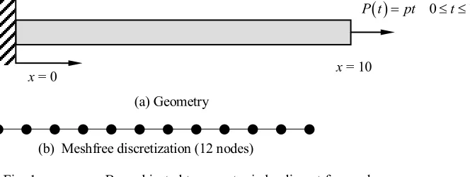
Consider a bar with length, L10 mm and cross sectional area, A1mm2 as shown in Fig. 1(a). Bar is
fixed at x0 mmand is free at x10 mm. A monotonic load, P t
pt 0 t 1, is applied at the free end of the bar, with p275 N. Material properties used in the numerical study are as follows:0 = 200
E GPa, = 10 h GPa, y = 250 MPa, = 0.06S , = 1s and, pD 0[1]. A typical meshfree discretization involving 12 uniformly spaced nodes is shown in Fig. 1(b). Modified exponential function with cˆ 2.7261 and
10
l is considered as the autocovariance function for initial damage field. For SF method random field discretization is chosen to coincide with meshfree discretization (i.e. M 12) whereas for KL expansion method
4
M is considered. It is found that for same M value (M 12) the computational time taken by KL expansion for reproducing the second order statistics of input field is 1.22 times of that taken by SF method.
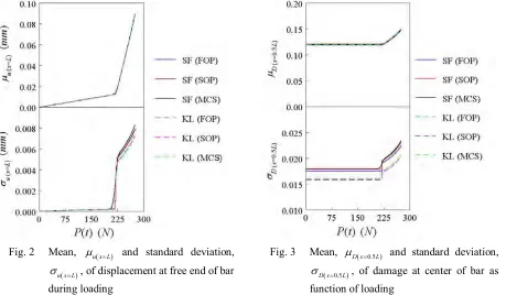
Fig. 2 shows the results of the mean, u x L and standard deviation, u x L , of the displacement at the free end of the bar during loading. The results of FOP, SOP, and MCS with 5000 samples, obtained using both SF and KL expansion methods are presented. The perturbation results of the mean, u x L and standard deviation, u x L
obtained using both methods matches well with corresponding MCS results. The values of standard deviation,
u x L
obtained using the KL expansion is lower than that obtained using SF method, especially in the plastic region (post yielding part of the curve). MCS results of the mean, u x L and standard deviation, u x L show smooth variation from elastic to plastic regime, since Monte Carlo technique can simulate different initial damage values along the length of bar for each simulation leading to nonuniform yielding of bar over the length. However FOP and SOP methods fail to capture this smooth variation, since perturbation method is based on Taylor series expansion at the mean values of homogeneous random field.
Fig 3 shows the results of the mean, D x 0.5L and standard deviation, D x 0.5L, of damage at the center of the bar as function of loading. Regardless of the method adopted for random field discretization, both FOP and SOP
Fig. 1 Bar subjected to monotonic loading at free end (b) Meshfree discretization (12 nodes)
(a) Geometry
x = 0 x = 10
0 1damage growth and hence there is no change in the mean, D x0.5L of damage, however, as the point under consideration starts to yield, it starts to grow nonlinearly. When compared with SF method, KL expansion method yields lower bound estimates of the standard deviation, D x 0.5L of damage, even though for both the cases FOP and SOP results match well with the corresponding MCS results.
Example 2: Plate with Hole under Tension
Square plate with circular hole under far field tensile loading as shown in Fig. 4(a) is considered. Plate dimensions are as follows: 2L40 mm and 2a2 mm. A monotonically increasing uniformly distributed load with p200 N is applied as shown in Fig. 4(a). Due to symmetry only one quarter of the plate is analyzed. A typical meshfree discretization involving total of 153 nodes is shown in Fig. 4(b). Modified exponential autocovariance function for two dimensions as defined in
0 0
2
1 1 1 2 2 2 1 1 1 2 2 2
ˆD D exp c lˆ c lˆ 1 c lˆ 1 c lˆ
Γ ζ ζ ζ ζ ζ with cˆ 2.7261 , cˆ 1.7262 and l l1 2 10 is
considered. In the present example M6 is used for the KL expansion method. In the SF method random field discretization, M 153 coincident with stress analysis nodal discretization is adopted.
Fig. 2 Mean, u x L and standard deviation,
u x L
, of displacement at free end of bar during loading
Fig. 3 Mean, D x 0.5L and standard deviation,
0.5
D x L
, of damage at center of bar as function of loading
0 2 0
0 .0 0 2 0 .0 0
(a) Geometry (b) Meshfree discretization (153 nodes)
0 1
P t pt t
x1 x2
2L 2L
Fig. 4.22 shows the results of the mean, D1.0003,0.0039 and standard deviation, D1.0003,0.0039, of damage at (1.0003, 0.0039) of the plate with hole as function of loading. Even though, FOP results match well with the corresponding MCS, KL expansion method underestimates the standard deviation, D4.97,4.97.
CONCLUSIONS
A stochastic EFGM is developed for the coupled elastoplastic damage analysis of structures with random initial damage. Damage is modeled as homogeneous random field. First and second order perturbation methods are derived to predict the mean and covariance properties of stochastic responses with, SF and KL expansion methods, as random field discretization techniques. Numerical examples comprising of one and two dimensional problems are solved to illustrate the effectiveness of the proposed method. MCS is used for validating the proposed method. A good agreement is observed between the results of the perturbation methods and MCS. However, perturbation methods fail to capture the smooth variation of statistical parameters of responses from elastic to plastic regime. Stochastic analysis shows that perturbation methods give convergent solutions of random responses for both the discretization schemes used. The KL expansion, though it is computationally effective, yields lower bound estimates of the second moment statistics.
REFERENCES
[1] Arun, C. O., Rao, B. N., Srinivasan, S. M., “Continuum Damage Growth Analysis Using Element Free Galerkin Method,” Sadhana, ,Vol. 35, Part 3, 2010 ,pp. 279-301.
[2] Kim, H.M. and J. Inoue, A Spectral Stochastic Element Free Galerkin Method for the Problems with Random Material Parameter. International Journal for Numerical Methods in Engineering. 61. 2004, 1957-1975. [3] Lancaster, P. and K. Salkauskas, Surfaces Generated by Moving Least Squares Methods. Mathematics of
Computation. 37, 1981, 141-158.
[4] Lemaitre, J. and R. Desmorat. Engineering Damage Mechanics. Springer-Verlag. 2005.
[5] Li, C. C. and A. Der Kiureghian, Optimal Discretization of Random Fields. Journal of Engineering Mechanics. 119. 6, 1993, 1136-1154.
[6] Rahman, S. and B.N. Rao A Perturbation Method for Stochastic Meshless Analysis In Elastostatics.
International Journal for Numerical Methods in Engineering. 50, 2001, 1969-1991.
[7] Rahman, S. and H. Xu, A Meshless Method for Computational Stochastic Mechanics. International Journal of
Computational Methods in Engineering Science and Mechanics. 6, 2005, 41-58.
[8] Sivakumar, M.S. and G.Z. Voyiadjis, A Simple Implicit Scheme for Stress Response Computation in Plasticity Models. Computational Mechanics. 20, 1997, 520-529.
[9] Spanos, P.D. and R.G. Ghanem, Stochastic Finite Element Expansion for Random Media. ASCE Journal of
Engineering Mechanics. 115. 5,1989, 1035-1053.
[10]Spanos, P.D., M. Beer, and J. Red-Horse, Karhunen-Loéve Expansion of Stochastic Process with a Modified Fig. 5 Mean,