Properties of statistical tests of neutrality for DNA polymorphism data.

Copyright 0 1995 by the Genetics Society of America

Properties of Statistical Tests of Neutrality for DNA Polymorphism Data

Katy

L. Simonsen,*

Gary

A.

Churchill*.+

and

Charles F.

Aquadro:

*Center for Applied Math, iBiometrics Unit, :Section of Genetics and Development, Cornell University, Ithaca, New York 14853

Manuscript received February 13, 1995 Accepted for publication June 9, 1995

ABSTRACT

A class of statistical tests based on molecular polymorphism data is studied to determine size and power properties. The class includes TAJIMA’S D statistic as well as the D* and F* tests proposed by Fu

and LI. A new method of constructing critical values for these tests is described. Simulations indicate that

TAJIMA’S test is generally most powerful against the alternative hypotheses of selective sweep, population bottleneck, and population subdivision, among tests within this class. However, even TAJIMA’S test can detect a selective sweep or bottleneck only if it has occurred within a specific interval of time in the recent past or population subdivision only when it has persisted for a very long time. For greatest power against the particular alternatives studied here, it is better to sequence more alleles than more sites.

G

IVEN a set of aligned DNA sequences from a sam- ple of n individuals of the same species, we would like to make inferences about the evolutionary history of the species. The neutral equilibrium model of se- quence evolution is often considered as a null hypothe- sis against which specific alternative models can be com- pared. The neutral hypothesis is rejected if the observed data are unlikely to arise under this model. A problem of interest is to construct appropriate test statistics that

will reject the neutral model with high probability when specific alternative models hold. We consider a class of test statistics that includes TAJIMA’S D statistic (1989a) and the

P

and E“ tests proposed by FU and LI (1993). The power properties of these tests against specific al- ternative hypotheses are studied using simulated data to determine how often and under which alternatives each test is able to reject the neutral model.

Critical values (rejection regions) of statistical tests are determined by the distribution of the statistics un- der the null hypothesis. The distributions of the test statistics we wish to examine are not known, but we can sample from these distributions by simulating data from the neutral model. Estimating the critical values is com- plicated because the distributions depend on the un- known value of a parameter

8

which is proportional to the product of the effective population size and the mutation rate.

Our goal is to determine which statistical tests are most powerful against different alternatives and to de- termine the sample sizes necessary to achieve a reason- able power. We also address the issue of larger sample sizes vs. greater number of sites sequenced with respect to improving statistical power.

Curresponding author; Katy Simonsen, Center for Applied Math, En- gineering and Theory Center, Cornell University, Ithaca, NY 14853. E-mail: [email protected]

Genetics 141: 41.3-429 (September, 1995)

This work was motivated in part by studies of natural populations of Drosophila. These studies have shown that levels of DNA polymorphism observed for a gene region are strongly correlated with regional rates of recombination, (e.g., AGUADE et al. 1989; STEPHAN and LANGLEY 1989; BEGUN and AQUADRO 1991,1992; BERRY et al. 1991; AQUADRO et al. 1994). One hypothesis to explain this correlation is that hitchhiking associated with the fixation of advantageous mutations leads to a reduction in linked neutral variation, (e.g., KAPLAN et al. 1989; MAYNARD SMITH and HAIGH 1974). However, in many of the cases cited TAJIMA’S D test did not reject the neutral model. This suggests the following question: is TAJIMA’S

D

powerful enough to detect deviations from the neutral model or is its behavior indistinguishable from neutrality even when the neutral model is vio- lated? The hitchhiking effect is simplest in the total absence of recombination when all variation at a locus is eliminated due to the fixation of a completely linked, advantageous mutation. Such a “selective sweep” event is one of the alternative hypotheses we investigate here. It must be emphasized that it is not the goal of the present paper to accept or reject the hitchhiking hy- pothesis for particular data sets. To do that, it would be necessary to set up hitchhiking as the null hypothesis and to explore the full range of possible parameters (including strength of selection, recombination rate, population size, dominance, neutral mutation rate, time since fixation) affecting this model. Here we vary only a few of these parameters to construct different alternative hypotheses against which the power can be estimated.

414 K. L. Simonsen, G. A. Churchill and C. F. Aquadro

test statistics and a method by which critical values for statistical tests of the neutral model can be obtained; then, we describe how data was simulated under alterna- tives to the neutral model. The RESULTS section summa- rizes the outcome of these simulations, showing the effect of these alternatives on the distributions of the test statistics and their power. In the final section, we discuss the implications of these results to performing statistical tests.

The neutral model: The neutral data were generated according to the coalescent model as described by HUD- SON (1990,1993). This model is based on the standard Wright-Fisher model and makes the following assump tions: ( 1 ) a large constant diploid population size of N individuals or 2N alleles (where

fl

%

N)

, (2) random mating, (3) nonoverlapping generations, (4) no recom- bination, and (5) an infinite-sites, constant rate neutral mutation process whereby an offspring differs from its parent allele by a Poisson-distributed number of muta- tions with mean p.

Under these assumptions, the probability that two particular individuals have the same parent in the previ- ous generation is 1/2N. The probability that any two individuals in a sample of size

j

have the same parent is

p

=

(4)

/2N. Thus, for a sample of j individuals in the current population, the probability that the first coales- cent event between any two of them occurs exactly t

+

1 generations ago is

p (

1 -

p)'.

That is, the time in

generations during which there are exactly j lineages in the genealogy of the sample is geometrically distributed with mean

l/p.

It is convenient to treat time as a contin- uous random variable. To this end, we approximate the geometric distribution with an exponential distribution with the same mean, because

p (

1 -

p)'

=

pe?' for small

p

and large t. The assumption (1) that

M2

% Nensures that

p

is sufficiently small. It is also convenient to mea- sure time in units of 2N generations, with the result that

p

is replaced by

(4).

Thus the time tj in units of 2N generations during which there are exactly

j lineages is

exponentially distributed with mean 1/($). The total time in the tree, T,,,, is equal to Cy=, jt,.

The number of mutations that occur on a lineage of length t is, by assumption ( 5 ) , Poisson-distributed with mean 2Npt = 8t/2, where 0 = 4Np. The assumption of infinite sites ensures that each mutation is observed as a polymorphic or segregating site. Therefore the num- ber S of segregating sites in a sample is Poisson-distrib- uted with mean 0T1,,,/2.

As HUDSON (1993) has pointed out, the fact that the true value of 0 for data sets is unknown presents a prob- lem when using simulation to estimate critical values for a test. Three methods of generating data are de- scribed by HUDSON (1993): conditioning on 8, condi- tioning on 8 and S, and conditioning on

S.

The first method is the one consistent with our model, but it requires knowing 0. The other two methods would re-

quire modifymg the null hypothesis: instead of a neutral mutation process with rate p, we would have to postu- late a fixed number of mutations that is independent of the total time in the tree. To apply the first method, we use the information contained in

S

to compute a range of values for 8 that are consistent with the ob- served data. We then use values of 8 in this interval to simulate the test statistic under the neutral model, and thus obtain critical values.

MATERIALS AND METHODS

Statistical tests

From n nucleotide sequences, statistics such as S, the num-

ber of segregating sites, k, the average number of painvise differences, and q,, the number of singletons (mutations ap- pearing in only one sampled allele), may be calculated. These are random variables whose distribution depends on a param- eter Q whose value is unknown, and each provides an unbiased estimate of 8. Let

n-l 1 n-' 1

a n =

C

7 , b,=

C

7 . (1)

,=I r = l

Under the neutral model, E(S) = anQ, E(k) = 0, and E ( q J = [ n/ ( n - 1)

3

0. Their variances are

Var(S) = a,@

+

b,02 (WATTERSON 1975) (2)

Var(k) = ~

( n

+

I ) Q + 2(n2

+

n

+

3)02

3 ( n - 1) 9n(n - 1)

(TAJIMA 1983) (3)

Var(qJ = - n

n - 1 n - 1 (72- 1 ) 2

(Fu and LI 1993). (4)

Therefore, S/a,, k, and [ ( n - 1 ) /n] q s are unbiased estimators of 8, and

m: = S ( S - l ) / ( &

+

b,) ( 5 )

d z

3nk(3(n - l ) k - n - 1)

l l n 2 - 7n

+

6

are unbiased estimators of 0'.

In the following section we define a class of test statistics that includes three previously described test statistics and six new ones.

Test statistics: From the three statistics S, k, and qs, we can calculate test statistics such as those of TAJIMA (1989a):

and of FU and LI (1993):

S / a , -

%(")

Power of Tests of Neutrality 415

W k , S, 71,) = (10)

LG-a

where the coefficients u and v are given in the APPENDIX. w e refer to the coefficients for TAJIMA’S statistic as uT and vT

rather than uD and uD to distinguish them from those for Fu and LI’S D statistic (1993), which is not studied in this paper because it requires an outgroup. The formula for up given in the APPENDIX differs slightly from that given in Fu and LI (1993, unnumbered equation p. 702) due to a typographical error in their paper. Under the neutral model the three sta- tistics D, L F , and F* all have expected value approximately 0 and variance approximately 1.

Each of these statistics is constructed in the same way. Un- der neutrality, the three quantities S/a,, k, and

vs[

( n

-

1 ) / n] all have expected value 8. Thus the difference between any two of these statistics will have expected value 0. The variances of the differences are of the form ye

+

E O 2 , where

y and E depend on the statistic in question. The variance of

the difference is estimated using S / a , and

rn;

as unbiased estimates for 8 and 02, respectively. The result is an estimated variance of the form US

+ vS2

where u = y / a , - v and v =

E /

( d

+

b,). Each test statistic is constructed by dividing the

difference by the square root of its estimated variance. Note that because this denominator depends on the data, the ex- pected value of the statistics is not exactly 0; simulations show that the mean is slightly negative. Because it is possible for the denominator to be 0, for purposes of this study we define D,

P,

and F* to be 0 when S = 0. This has the effect of making rejection of the neutral model impossible when no variation is observed.

The statistics D, L F , and F* use S and

rn;

to estimate 8 and

8‘ in the variance term y e

+

EO’. It is also possible to use k and

4

or

vs

and

4

to make this estimate. S has been used because S/a, has a smaller variance under neutrality than the other possibilities. In nonneutral situations, however, the be- havior of S, k, and 7, is more complex, so that k or 71, could make a better estimator of 8 or O2 in some cases. We can construct six new test statistics, as follows

k - S/a,

Tz(k, s) = (11)

G ( k ,

s,

71,) = k

- S/a,

(12)

JUT371,

+

VT$

S/a, -

v3(

e)

@(k,

s,

173

= (13)

S/a, - 7,

n-l

@(St 71s) = ( n )

(14)

JUd7IS

+

vLg7I:

k -

%(e)

G(k,

7s) =

& G g s

k -

71~(%)

G(k,

71,) =

J U F m + vqv:

The subscript 2 or 3 indicates that the estimate of 8 uses k and Q , or q, and %, respectively. The coefficients u and v

are defined in the APPENDIX. The properties of these tests will be investigated along with those of the standard tests. For convenience, we again define these statistics to be 0 when their denominator is 0.

Hypothesis testing issues: Because neither S, k, nor q s is a sufficient statistic for 8, the variance of any of the above test statistics will not be one and will vary with 6’ (HUDSON 1993). Thus, computed critical values for these test statistics must account for the unknown 8. Furthermore, even when 8 is known, the exact distribution of the statistics under the null hypothesis is not. To perform twmided tests of level a , the critical values required are the boundaries of a (1 - a ) confi- dence interval for the test statistic. That is, for the statistic D we require Da and DL, independent of 8, such that the sum

of the pvalues pL = ProbH, (D 5 DL) and pa = Prob, (D 2

Da) is less than or equal to a . We note that because S, (2“) k, and 77 are integers, the test statistics will have a discrete distri- bution, and so any non-randomized test will not precisely achieve the desired level. Other authors have suggested meth- ods to determine critical values as described below. We pre- sent an alternative method.

TAJIMA (1989a) computed critical values by assuming D to have a beta distribution with mean zero and variance one, scaled to the interval [Dmin, Dm,]. TAJIMA’S justification is based on a visual comparison between beta densities and his- tograms of simulated data. We have found that TAJIMA’S criti- cal values are often too conservative, particularly at the upper tail of the distribution. While it is true that the probability of false rejection is not increased by using conservative critical values, it can result in a serious reduction in power. Thus this method of obtaining critical values is less than satisfactory.

Fu and LI (1993) used simulated data with known values of 8 and n to locate appropriate percentiles as estimates for the critical value of the statistic. Then for each value of n, they took the most extreme of these critical values over all 8’s in the interval [2, 201. The effect of this technique is to reject only when the data cannot be explained by neutral evolution for any value of 8 in this interval. The interval [2, 201 for 8 was chosen somewhat arbitrarily to represent “most cases of interest.”

While FU and LI’S approach is an improvement over TAJI-

MA’S, there are still some problems remaining. First, the criti-

cal values are not applicable when the true value of 6’ is not in [2,20], and we cannot know, for a given set of data, whether this is the case. Because 0 is a per-locus value, it changes with the number of nucleotides being sequenced, as well as with the underlying mutation rate. Thus it is difficult to justify why

8 would have to be confined to this range. The test may falsely reject when 8 is not in this interval. Further, their technique does not take into account the information about 8 inherent in the data. We will attempt to address these problems below. The problem of the unknown parameter 8 may be ad- dressed using the technique proposed by BERCER and Boos (1994). Ideally, we would like to reject only if the data cannot be explained by any positive value of 8. For a test of level a

this would mean choosing critical values [ D , ~ , Du] for D such that

@€[OF)

sup [Probe@ 5 DL)

+

Prob#(D 2 Du)] 5 a (17)

However, we cannot perform simulations for infinitely many values of 8, nor is it reasonable to do so because extremely large values of 8 are unlikely. Instead, for some small number

p

< a , we use the data to estimate C,, a 1 -

p

confidence

416 K. L. Simonsen, G. A. Churchill and C. F. Aquadro

sup[Probn(D 5 DI.)

+

Probo(D 2 Du)] 5 cy -

p.

(18)

n E c,

For each 8 in a grid covering C, we estimate level (a -

0)

critical values [L$, &] using the percentiles of neutral data for that 8. We take the most extreme of those critical values over all 8 in C,:

Dl> = min D;,, Dc, = max

Dt.

(19)

nE co BE co

The result is a level a test, as shown by BERGER and BOOS

(1994). This approach is similar to that of Fv and Lr (1993), except that instead of arbitrarily using the interval [2, 201 we use an interval that reflects our knowledge of 8 for the data set being considered. This has the advantage of giving us a test with known level for any value of the unknown parameter 8.

To construct this 1 -

p

confidence interval for 8, we use the exact distribution for S given 8, as given by T A V ~ (1984). We wish to find a two-sided interval C, = [ S ,

e,]

such that, for a particular observation S = s, and for fixed n,

Prob(S 2 s i 8 = 8,) =

p/2

(20)

Prob(S 5 510 =

e(,)

= p/2. (21)

The cumulative distribution function for S given 8 is

F(s, n, 8) = Prob(S 5 518)

So, (20) and (21) may be written as

F(s - 1 , n, 0,) = 1 - p/2 (231

m , n, 0,) =

p/2

(24)

Thus we must solve (23) and (24) for Or, and OU for the particular values of S = 5 and n observed in the data. This is

computationally intensive for large values of n and requires high precision to compute accurately in many cases. We used the variable-precision capabilities of the symbolic computa- tion package Maple (CHAR et al. 1991) to perform the calcula- tions. The results of these computations are given in RESULTS.

Note that when S = 0 is observed, it is appropriate to set Or = 0 and solve F(0, n, 0,) = ,8 for OUin place of (24); however, because all the test statistics are defined to be 0 in this case, the resulting critical values will be irrelevant.

In summary, there are three distinct steps to computing critical values for the test statistics in this fashion. (1) For the values of n and S required, compute C,, a 1 - ,8 confidence

region for 8 given S. (2) For a grid of 8 values in C, and for each n, simulate a large number of samples and estimate level (a -

p )

critical values for each test statistic from the simulated empirical distributions. ( 3 ) Take the maximum upper critical value and minimum lower critical value over all values of 8 in C , , for each value of n and S and for each test statistic. This gives critical values of a-level tests for each n and S.

Simulations

To evaluate the power of the statistical tests described above, we require data simulated under a number of different alternative models. The alternatives considered here: a selec- tive sweep event, a population bottleneck, and a subdivided population, represent a few simple deviations from strict neu- trality and are meant as examples rather than as a comprehen- sive study. Because balancing selection is similar to population subdivision from a coalescent perspective (HUDSON 19901, we

MRcAA

I

past

/ \ I t

1 2 3 4 5 present

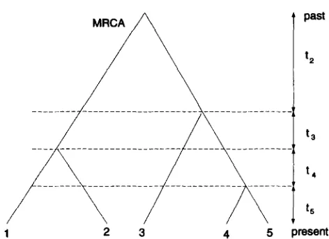
FIGURE 1.-An example of a coalescent tree for a sample of five alleles.

expect the results for a subdivided population to be applicable to the corresponding balancing selection alternative as well.

Neutral simulations: A sample of DNA sequences is gener- ated by simulating a random gene genealogy according to

the algorithm developed by HUDSON (1990, 1993). There are three components to this genealogy: topology, branch lengths, and mutations. First, a random tree topology is gener- ated for the genealogy. From n individuals in the sample, two are chosen at random to be the first to coalesce. A new individual is designated as their parent, and the process is repeated on the remaining n - 1 individuals. The process stops when only one individual, the most recent common ancestor (MRCA) of the entire sample, remains. This gives the topology of a binary tree with n tips. Next, the branch lengths are chosen:

4,

the time (in units of 2N generations) during which there are exactly j lineages, is an exponentially distributed random variable with mean 1/({) as described in the Introduction. These two steps define a tree such as that shown in Figure 1. Finally, mutations are added to the tree. The number of mutations S that have occurred during the history of the sample is generated as a Poissondistributed random variable with mean 8Ttot/2. For each mutation, the branch of the tree on which it occurred is chosen randomly, where the relative probability of each branch is proportional to its length. The mutation is transmitted to each offspring descended from that branch. Thus each individual is assigned a "sequence" of nucleotides designated, for example, -+--++-,where "-" indicates that the nucleotide is iden- tical to the ancestral sequence at that site and

"+"

indicates a mutation. Under the infinite-sites model, each mutation is assumed to take place at a distinct nucleotide site, and thus each sequence generated is composed only of polymorphic or segregating sites.

Selective sweep simulations: A highly favorable mutation with selective advantage s and dominance h that occurs at a time T, is assumed to sweep through the population and reach fixation in a deterministic fashion, such that the proportion

x ( t ) of individuals carrying the mutation at time t follows PNs.41 - X)[X

+

h(1 - ZX)] 1

X ( t ) =

Power of Tests of Neutrality 41 7

when the frequency is low, and that the allele has been fixed in the population when the frequency reaches 1 - 1/2N.

The selective sweep alters the coalescent process by reduc- ing the effective population size of the parental generation at time t from 2N to 2Nx( t), because only genes carrying the selected mutation may be chosen as ancestors of the sample. The per-generation coalescent probabilities change from (4)/2N to (4)/[2Nx( t)]. Thus the total size of the tree is re- duced, and the effect of the selective sweep is to reduce varia- tion at and around the selected locus. We are assuming no recombination between the selected and sampled loci.

To generate coalescent times under a sweep, we generate times according to the neutral model, and then scale them appropriately, as described below. This approach was sug- gested to us by R. R. HUDSON; also see GRIFFITHS and TAVAR~ (1994, equation 3). To convert a time from one time scale to another, we must perform a change of variables. Suppose U is a time measured in units of 2Nx(t) at time t. We wish to convert this time Uback into the standard units of 2Ngenera- tions. The instantaneous change of variables at time t is 2Nx(t)du = PNdt, where dt is the interval in regular units 2N and du is the time interval in units 2Nx(t). This becomes

and thus, if T represents the same time as U but in regular units, we integrate over the whole interval to obtain

Therefore, to generate a coalescent time T under a selective sweep described by x ( t ) , we generate a time U under the neutral model and then find Twhich solves (27). This is done for each coalescent time in a tree, to generate a coalescent tree for a selective sweep.

If the selective sweep began quite recently, it is possible that the selected allele has not yet been fixed in the popula- tion. The length of time Td this sweep takes to complete de- pends on N, s, and h; for example when h =

'/*,

the sweep lasts Td = 2 ln(2N - l ) / s N If T, > Td, then the allele has

become fixed by the present time (0), and so the MRCA of the sample has to occur more recently than T,, because it must be descended from the initial selected mutant. If the sweep began so recently that the selected allele has not yet completely reached fixation (T , < T d ) , then there are two

types of alleles in the present population, those with, and those without, the selected mutation, in the ratio x(0):l - x(0).

In this case we assume the number of sampled individuals having the selected mutation is binomially distributed with parameters (n, x(0)). The selected alleles follow the above sweep model, while the rest of the sample is drawn from a population of size 2N[1 - x ( t)] at time t. This requires a shift in time units similar to that described above, with x(t) re- placed by 1 - x( t ) . Before the selected mutation occurred, ( t > Ts) all ancestors follow a neutral model.

Our model of the selective sweep is defined in terms of four parameters: h, s, N, and its starting time T,. For this study, we chose to fix h = 0.5, N = lo6, and s = and allow T, to vary over the range 0-2 (in units of 2N, back in time from the present). This is relatively weak selection on a codominant allele; for comparison we also performed the simulations with

s =

lo-*.

For combinations of n (10, 20, 50,

loo),

0 (10, 20,

50), and T, (in increments of 0.01 from 0 to 0.3, then in increments of 0.05 from 0.3 to 0.5, then in increments of 0.1 from 0.5 to 2.0), 5000 samples were generated and the proportion of rejections for each of the tests recorded.

A selective sweep is expected to reduce polymorphism at linked sites, because any observed polymorphism must be the result of mutations that have occurred since the sweep. These newly arisen mutations will at first be rare and will increase in frequency as the time since the sweep increases. Because S takes into account only the number of mutations, while k is also affected by their frequency, it is expected that S will recover more rapidly than k from the effects of a sweep. This will have the effect of reducing the expected value of TAJIMA'S statistic below its neutral expectation of 0. The magnitude of this reduction has not been predicted by theory, and is one of the subjects of the present investigation.

Population bottleneck simulations: A population bottle- neck is assumed to occur when the population, originally of size 2N, is suddenly reduced to a fraction f of its former size for a length of time I, then instantaneously regains its initial size. Let Tb be the time (in units of 2N generations) at which the bottleneck ended, so that it began at a time Tb

+

I, which is further from the present time 0. Coalescent times under this model are obtained by scaling neutral coalescent times in the same way as the selective sweep. In this case, the changing population size 2Nx( t) is a step function rather than a smooth curve as it was for the sweep, so the integration in (27) is easy. We generate a time u, under the neutral model, and then use as the coalescent time

5

given by

This is equivalent to the following probability density for the coalescent times t,:

where p =

(4).

The density can be derived by considering the per-generation probabilities of coalescence during the three stages of the bottleneck.

For purposes of this study, we kept f fixed at 0.01, 1 fixed at 0.1, and varied Tb, the time since the bottleneck ended, from 0 to five. These are bottlenecks of the same severity but lasting ten times the length of those considered by TAJIMA (1993). The fraction rejected out of 1000 simulations was recorded.

A population bottleneck is expected to reduce polymor- phism throughout the genome, because a drastic reduction in population size is likely to eliminate many rare variants. As in the case of the selective sweep, most of the polymorphism will be a result of new mutations, which will be rare. Thus a reduction of unknown magnitude in the expectation of TAJI-

MA'S statistic is predicted (1989b).

418 IC L. Simonsen, G. A. Churchill and C. F. Aquadro

respectively, which evolve independently from then on. Here, the sample of n alleles consists of nA alleles of type A, and nB

of type B, with n = nA

+

nB.

The coalescent tree for such a subdivided population is generated in the following manner. As usual we work back- ward in time from the present to the time of the MRCA of the sample. Let j A and j B be the number of lineages of type

A and B remaining at any given time. Initially, we let j A = nA and jB = nB, and at each coalescent event, one of them is decremented. We need to know the distribution of the time back to the next coalescent event.

In the subdivided model, the coalescent probabilities be- fore and after the population split are different. When the two populations are disjoint, the probability per generation that two A individuals coalesce is

PA

= ( $ ) / 2 N A while for the B population it is pB = (li5)/2NB. The probability that both populations will coalesce in the same generation is negligible [ O ( l / P ) ] compared with

PA

and

pB,

and so the per-genera- tion probability of a coalescent event in either population is approximately pl =

PA

+

pB

while the two populations are disjoint. When the two populations are mixed, we have a single population of size 2NAB, with j A

+

j B sample lineages present. Thus the per-generation probability of coalescence for the mixed population is P, = (j49/2NAB.

As before, t, is the time during which there are exactly i lineages of any type present. Let S, = t,, with S,+, = 0. S,

keeps track of the total time generated so far. To generate the time $A+jB to the next event, it is necessary to know the

relationship between SjA+j,+l and T,. In particular, if SjA+JB+l > T,, then we have passed the subdivision point and we may generate subsequent times

5A+lB

simply as exponentially dis- tributed random variables wth parameter

p .

On the other hand, suppose SjA+JB+l

<

T,, say T, - $A+jlr+l = M > 0. Then

the time $A+jB generated could be less than or greater than

M. The probability of coalescence after a given time t < M is (1 -

pl)'fi

= ple?I'. But for a time t > M, the robability of coalescence is (1 -

p,)"(

1 -

p)'"p

=

p$"""

J

( t ' x - p l ) . Thus

where I is an indicator function and M = T, -

Once a time has been generated from this mixture of expo- nentials, two individuals must be chosen to coalesce at that time. If the total time

4A+j,+l

is still less than T,, then we must choose between group A and group B with relative probabili- ties

PA

and pn. If the time is greater than T,, we have only one group. Once the group is chosen, two of the appropriate group are selected at random, and the corresponding j is decremented. The process is repeated until only one individ- ual remains.

When a population is subdivided, the average pairwise dif- ference k is inflated relative to the total number of mutations

S, because of the large divergence between subpopulations. Thus the qualitative expectation is that D will have a positive mean in this situation. As with the selective sweep and bottle- neck, we chose time since the subdivision event as the primary variable to investigate, fixing NA = NB = NAB/2, nA = nB =

25. and 0 = 20.

RESULTS

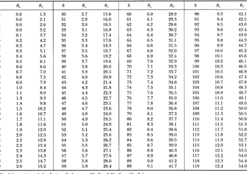
Results of neutral simulations: Simulations of the null hypothesis were used to provide new critical values for the test statistics. Our technique uses confidence intervals for 8 given S, as described in MATERIALS AND

METHODS. These 1 -

p

confidence intervals were com- puted using 40 digits of accuracy to solve equations 23

a n d 24. Tabulation here of these confidence intervals for different values of n, S, and

p

would be prohibitive, so we show only a sample: the case n = 50,

p

= 0.01 in Table 1. This table shows, for example, that if S = 23

is observed from a sample of size n = 50, and the neutral model holds, then with 99% certainty 8 is between 2 and 12.5. For other values of n a n d

p,

O L a n d 8, may be closely approximated by linear functions of S, especially when S is large. For example, when n = 20, Co.ol

=

[0.121S- 0.481,0.709S+ 2.8581 and Co.ool

=

[O.O94S- 0.473, 0.904s

+

4.4181. T h e coefficients of these linear approximations are given in Table 2, and can be used to approximate the values corresponding to Table 1 for other values of n a n d

p.

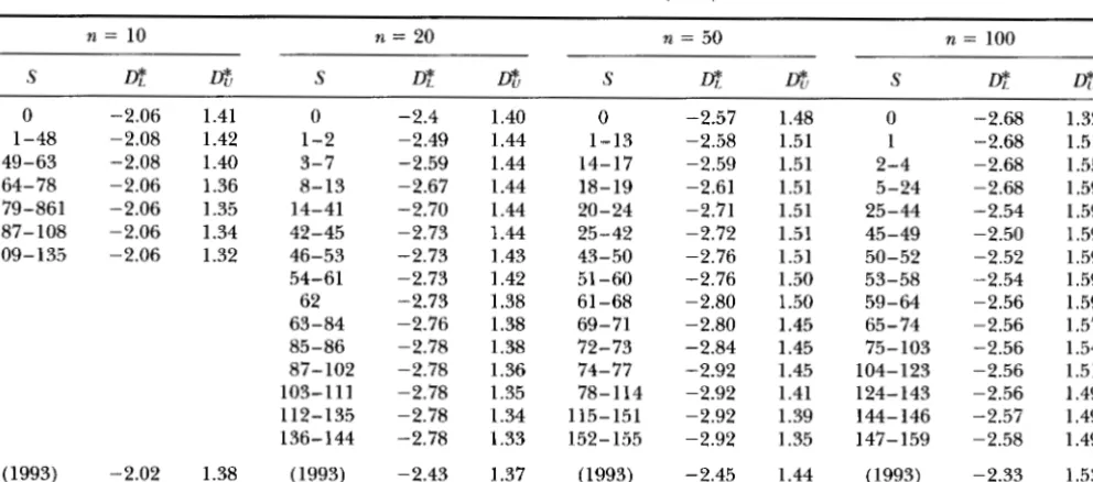
Table 3 shows tables of level 0.05 critical values for

TAJIMA'S test for a range of Svalues, for n = 10, 20, 50, 100, using (Y = 0.05 a n d

p

= 0.01. For comparison, the values from the beta distribution (TAJIMA 1989a) are also shown. Corresponding values for

LY

and

P

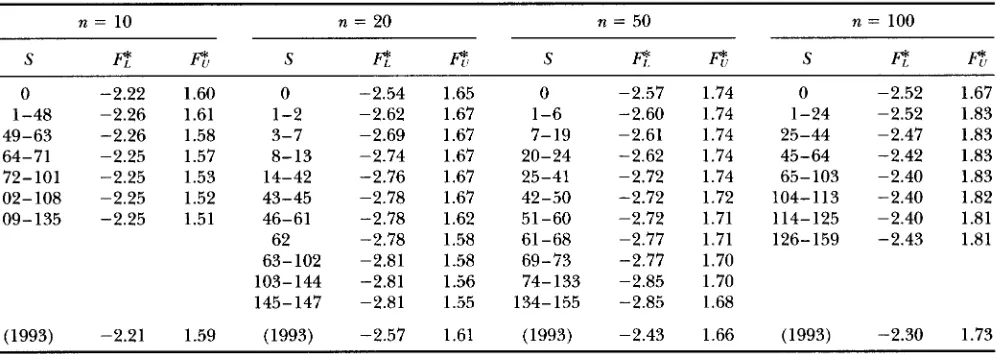
(Fu a n d LI 1993) are given in Tables 4 a n d 5 , along with the values that assume 8 E [2, 201 from (Fu and LI

1993).

There is n o simple pattern to the way in which the new critical values differ from those of the beta distribu- tion. Generally speaking, for small n the beta distribu- tion values are too large, while for larger n the beta distribution values are too small. The important differ- ence is that the new values are based on a sound statisti- cal framework that does not depend on fitting the statis- tic to a particular distribution, as TAJIMA did, or on the true value of

8

being between 2 a n d 20, as FU and LI assumed.

T h e size of these tests (the probability of rejecting when the neutral model is true), based on the new critical values, was estimated by applying each test to 10,000 simulated neutral data sets for each value of 8.

The number of false rejections was computed (data not shown). The size for most values of 8 is between 3 a n d 496, o u t of a maximum of (Y = 5%. This shortfall is attributable to three factors. First, because the statistics have discrete distributions, we cannot expect to pre- cisely achieve the desired level with any nonrandomized test. Second, there is some error in estimating the (a

-

0)

critical values using the empirical percentiles, be-

cause we used a finite number of simulations (10,000). This source of error could be diminished, though not eliminated, by using a larger number of simulations. Third, the Berger a n d Boos confidence interval proce- d u r e is conservative; using it may reduce the size of the test by as much as

p.

Our choice of was arbitrary, and the effect of this choice on the size of the tests is not clear. Thus, the critical values might be improved by

using a different value of

p.

Power of Tests of Neutrality

TABLE 1

The 99% confidence intervals for 8

419 0 1 2 3 4 5 6 7 8 9 10 11 12 13 14 15 16 17 18 19 20 21 22 23 24 25 26 27 28 29 0.0 0.0 0.0 0.0 0.1 0.2 0.3 0.3 0.4 0.5 0.6 0.7 0.8 0.9 1

.o

1.1 1.3 1.4 1.5 1.6 1.7 1.8 1.9 2.0 2.1 2.2 2.3 2.4 2.5 2.6 1.3 2.1 2.6 3.2 3.7 4.2 4.7 5.1 5.6 6.1 6.6 7.0 7.5 7.9 8.4 8.9 9.3 9.8 10.2 10.7 11.1 11.6 12.0 12.5 12.9 13.4 13.8 14.3 14.7 15.2 30 31 32 33 34 35 36 37 38 39 40 41 42 43 44 45 46 47 48 49 50 51 52 53 54 55 56 57 58 59 2.7 2.9 3.0 3.1 3.2 3.3 3.4 3.5 3.6 3.7 3.8 3.9 4.0 4.2 4.3 4.4 4.5 4.6 4.7 4.8 4.9 5.0 5.1 5.2 5.3 5.5 5.6 5.7 5.8 5.9 15.6 16.0 16.5 16.9 17.4 17.8 18.3 18.7 19.2 19.6 20.0 20.5 20.9 21.4 21.8 22.3 22.7 23.1 23.6 24.0 24.5 24.9 25.4 25.8 26.2 26.7 27.1 27.6 28.0 28.4

S

4.

0"

60 61 62 63 64 65 66 67 68 69 70 71 72 73 74 75 76 77 78 79 80 81 82 83 84 85 86 87 88 89 6.0 6.1 6.2 6.3 6.4 6.5 6.6 6.8 6.9 7.0 7.1 7.2 7.3 7.4 7.5 7.6 7.7 7.8 8.0 8.1 8.2 8.3 8.4 8.5 8.6 8.7 8.8 8.9 9.0 9.1 28.9 29.3 29.8 30.2 30.7 31.1 31.5 32.0 32.4 32.9 33.3 33.7 34.2 34.6 35.1 35.5 35.9 36.4 36.8 37.3 37.7 38.1 38.6 39.0 39.5 39.9 40.3 40.8 41.2 41.7 90 91 92 93 94 95 96 97 98 99 100 101 102 103 104 105 106 107 108 109 110 111 112 113 114 115 116 117 118 119 9.3 9.4 9.5 9.6 9.7 9.8 9.9 10.0 10.1 10.2 10.3 10.5 10.6 10.7 10.8 10.9 11.0 11.1 11.2 11.3 11.4 11.5 11.7 11.8 11.9 12.0 12.1 12.2 12.3 12.4 42.1 42.5 43.0 43.4 43.9 44.3 44.7 45.2 45.6 46.1 46.5 46.9 47.4 47.8 48.3 48.7 49.1 49.6 50.0 50.5 50.9 51.3 51.8 52.2 52.7 53.1 53.5 54.0 54.4 54.9

Confidence intervals for 0 given Swhen n = 50, ,B = 0.01. C, =

[e,,

e,].

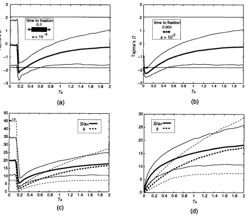
a selective sweep on TAJIMA'S D, S / a , and k is shown in Figure

2

for two different strengths of selection: s = (weak, a and c); s =

lo-'

(stronger, b and d); for 5000 simulations with n = 50 and 0 = 20. The horizontal axis is T,, the time at which the sweep began. Because the present time is 0, this is also the amount of time since the sweep began. In Figure 2, a and b, the thicker curve is the mean of TAJIMA'S D, while the thinner

TABLE 2

Coefficients of linear approximations to a

1-/3 confidence interval for 8

P

n b C q r

0.01 10 0.133 -0.484 1.236 3.787 20 0.121 -0.481 0.709 2.858 50 0.108 -0.474 0.441 2.302 100 0.101 -0.484 0.341 2.039 0.001 10 0.102 -0.483 1.782 6.304 20 0.094 -0.473 0.904 4.418 50 0.087 -0.468 0.519 3.408

100 0.081 -0.856 0.389 3.420

Co = [bS

+

C, qS

+

r ] .

curves are the

2.5

and 97.5 percentiles. For comparison, the critical values from TAJIMA'S (1989a) beta distribu- tion are also shown (horizontal lines), though the criti- cal values from Table 3 were used to determine rejec- tion. The expected trend towards more negative values of D is observed. There is also a pronounced decrease in the variance of the distribution even when the sweep is very ancient. When T, is very large (six or seven, not shown), the percentile curves eventually level off close to the critical values. Figure 2, c and d, show the values of S / a , (solid) and k (dotted) associated with a and b respectively. The thicker lines represent the means, while the thinner lines are the 2.5 and 97.5 percentiles. For large T, the means converge close to their neutral expectation of 0 = 20. It can be seen that a selective sweep affects k more strongly than S , and that k recovers more slowly both in mean and variance. Comparing Figure 2, a and c with b and d shows the effect of the strength of selection: stronger selection results in a more immediate decrease in the expected value of D,

and a stronger reduction in S and k. Note, however, that the length of time Td (=2 ln(2N) / N s when h =

420 K. L. Simonsen, G. A. Churchill and C. F. Aquadro

TABLE 3

Level 0.05 critical values of TAJIMA'S D test

0 1-26 27-41 42-48 49- 63 64-71 72-135

beta

-1.79 -1.80 -1.80

- 1.80

-1.79 -1.78

- 1.78

- 1.733 1.84 1.84 1.83 1.81 1.79 1.78 1.74

1.975

0 1-3 4-14 15-20 21-28 29-36 37-45 46-86 87-144 145-147

beta

-1.78 -1.82

- 1.83 - 1.84

-1.84

- 1.84

- 1.84

- 1.84

-1.85

- 1.85

- 1.803 1.97 1.97 1.97 1.97 1.96 1.90 1.88 1.87 1.87 1.82

2.001

0 1-22 23-31 32-41 42-50 51 -73 74- 155

beta

-1.70 2.11 -1.77 2.11 -1.77 2.06 -1.77 2.00 -1.73 1.97 -1.73 1.95 -1.75 1.95

- 1.800 2.044

0 1-24 25-34 35-44 45 - 74 75 - 78 79- 159

beta

-1.58 -1.70 -1.70 -1.70 -1.70 -1.68 -1.69

-1.781

2.21 2.21 2.15 2.07 2.04 2.01 2.01

2.073 Values based on a 99% confidence interval for 0 given S for several sample sizes n.

account; this is a 0 . 3 and 0.003 for the weak and strong cases, respectively (shown inset in Figure 2, a and b). Thus in a and c, when T,

<

0.3, the selected allele has not yet been fixed at time 0 when we take the sample. The apparently neutral behavior when T,

<

0.15 is due to the low frequency of the selected allele in the popula- tion, and hence a low probability that they will be found in the sample. When 0.15

<

T,

<

0.3, we see the effect of a selective sweep in progress, while when T,

>

0.3, we have the result of a completed selective sweep. In Figure

2,

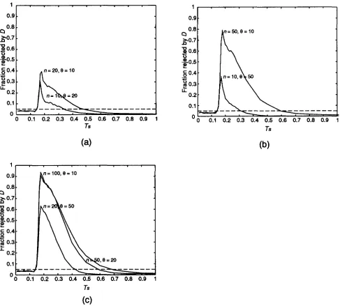
b and d, on the other hand, the sweep is virtually instantaneous compared with the scale shown (though it takes 6000 generations), so the effect is seen immediately.

The power of TAJIMA'S D test against the selective sweep alternative is shown in Figure 3: 8 = 10, s =

s =

lo-'

(d). The horizontal axis is T, as in Figure 2,

but note that the scale is enlarged. The different curves are for different values of n as labeled on the graphs. Figure 3 shows that the sample size has a profound effect on the power to reject. While a sample of size 50 or 100 can give a substantial power, no significant result can be expected from a sample size of 10 in most cases. It appears that even with large sample sizes, it is only possible to detect selective sweeps that occurred in a specific window of time. For example, if n = 100 and

8 = 20, TAJIMA'S test will reject with probability 90%

(a);

e

= 20, s =

iop4

(b);

e

= 50, s = 1 0 - ~ (c);

e

= 20,

TABLE 4

Level 0.05 critical values of FU and LI'S (1993) D* test

n = 10 n = 20 n = 50 n = 100

s

Le

@" S

@

OTi

S

Le

P

"

S

Le

a

0 -2.06 1.41 0 -2.4 1.40 0 -2.57 1.48 0 -2.68 1.32

1-48 -2.08 1.42 1-2 -2.49 1.44 1-13 -2.58 1.51 1 -2.68 1.51 49-63 -2.08 1.40 3-7 -2.59 1.44 14-17 -2.59 1.51 2-4 -2.68 1.55 64-78 -2.06 1.36 8-13 -2.67 1.44 18-19 -2.61 1.51 5-24 -2.68 1.59 79-861 -2.06 1.35 14-41 -2.70 1.44 20-24 -2.71 1.51 25-44 -2.54 1.59 87-108 -2.06 1.34 42-45 -2.73 1.44 25-42 -2.72 1.51 45-49 -2.50 1.59 109-135 -2.06 1.32 46-53 -2.73 1.43 43-50 -2.76 1.51 50-52 -2.52 1.59

54-61 -2.73 1.42 51-60 -2.76 1.50 53-58 -2.54 1.59

62 -2.73 1.38 61-68 -2.80 1.50 59-64 -2.56 1.59 63-84 -2.76 1.38 69-71 -2.80 1.45 65-74 -2.56 1.57 85-86 -2.78 1.38 72-73 -2.84 1.45 75-103 -2.56 1.54 87-102 -2.78 1.36 74-77 -2.92 1.45 104-123 -2.56 1.51 103-111 -2.78 1.35 78-114 -2.92 1.41 124-143 -2.56 1.49 112-135 -2.78 1.34 115-151 -2.92 1.39 144-146 -2.57 1.49 136-144 -2.78 1.33 152-155 -2.92 1.35 147-159 -2.58 1.49

(1993) -2.02 1.38 (1993) -2.43 1.37 (1993) -2.45 1.44 (1993) -2.33 1.53

Power of Tests of Neutrality 42 1

TABLE 5

Level 0.05 critical values of FIJ and LI’S F* test

n = 10 n = 20 n = 50 n = 100

S

E

f l l S

E

E

7

S

f l

f i

S

E

E

T

0 -2.22 1.60 0 -2.54 1.65 0 -2.57 1.74 0 -2.52 1.67

1-48 -2.26 1.61 1-2 -2.62 1.67 1-6 -2.60 1.74 1-24 -2.52 1.83 49-63 -2.26 1.58 3-7 -2.69 1.67 7-19 -2.61 1.74 25-44 -2.47 1.83 64-71 -2.25 1.57 8-13 -2.74 1.67 20-24 -2.62 1.74 45-64 -2.42 1.83 72-101 -2.25 1.53 14-42 -2.76 1.67 25-41 -2.72 1.74 65-103 -2.40 1.83 102-108 -2.25 1.52 43-45 -2.78 1.67 42-50 -2.72 1.72 104-113 -2.40 1.82

109-135 -2.25 1.51 46-61 -2.78 1.62 51-60 -2.72 1.71 114-125 -2.40 1.81 62 -2.78 1.58 61-68 -2.77 1.71 126-159 -2.43 1.81 63-102 -2.81 1.58 69-73 “2.77 1.70

103-144 -2.81 1.56 74-133 -2.85 1.70 145-147 -2.81 1.55 134-155 -2.85 1.68

(1993) -2.21 1.59 (1993) -2.57 1.61 (1993) -2.43 1.66 (1993) -2.30 1.73

Values based on a 99% confidence interval for 8 given S for several sample sizes n.

only if the sweep (weak selection) began between T, = 0.18 and T, = 0.27, which, with N =

lo6,

corresponds to between 360,000 and 540,000 generations ago. It must be emphasized that these results apply only to the particular model of sweep and the parameter values (s

= h = 0.5) used in the simulation. For clarity, the graphs in Figure 3 are shown with T, in the range 0- 1. However, simulations were actually performed with

T, as large as 10. It can be seen in Figure 3 that the power drops well below the neutral expectation of 0.05

when

T,

is close to one. In fact, a selective sweep reduces the power even when T, is four or five. For these T,, the sweep was long enough ago that new mutations have had a chance to reach intermediate frequency in the population, but polymorphism is still quite reduced. In other words, the difference between the expectations of k and S/u, is fairly small, but the variance of that difference is still reduced well below one. This has the paradoxical result of making the test less likely to reject under the alternative than under the null hypothesis, when T, takes on intermediate values. In other words, TAJIMA’S D test is biased.

Figure 4 shows the power of all nine tests against the selective sweep alternative when n = 50 and 8 = 20; s

= (a), s = lo-‘ (b). Among all the tests considered, TAJIMA’S test showed the most power against the selec- tive sweep for each value of n and

8

we simulated. The tests T2 and F3 were almost as powerful as D, and were more powerful than Fu and LI’S

P

and

LY

tests, Al-

though TAJIMA’S test statistic does lack power in many cases, it appears to be the most powerful test of this class against the selective sweep alternative as modeled here, both for weak and strong selection. We cannot, of course, generalize this result to any alternative hypotheses that we did not simulate, such as other val- ues of N, h, and s, or models of hitchhiking which allow

recombination, but lacking evidence to the contrary it would be reasonable to assume the result holds at least for parameters within the range of those used in the simulations, such as s between and lo-‘, and 8

between 10 and 50.

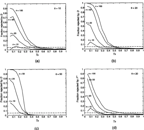
Results of population bottleneck simulations: The results for the population bottleneck are summarized in Figures 5 and 6. Each figure represents a bottleneck lasting 0.1 (units 2Ngenerations) and dropping to 1%

of its original size. The horizontal axis in each case is the time Tb at which the bottleneck ended, and each data point is based on 1000 simulations. Figure 5 shows the mean and 2.5 and 97.5 percentiles of TAJIMA’S statis- tic D, us. Tb, for n = 50 and 8 = 20. Figure 6 shows the fraction rejected by TAJIMA’S test for the cases 8 = 10 (a),

8

= 20 (b), 8 = 50 (c), and by Fu and LI’S

F*

test for the case 8 = 20 (d). The results are similar to those for the selective sweep. A bottleneck is only likely to be detected if it is very recent, and if the sample size is large. Again, TAJIMA’S test performs the best of all the tests considered. The similarity of the results to those for a selective sweep is to be expected, since the effect on the coalescent process of the two situations is similar. Results of population subdivision simulations: Popu- lation subdivision has an effect opposite to that of a selective sweep on the statistics being studied. A subdi- vided population results in a higher value of k than would be expected under neutrality, while the effect on S is less severe. Thus population subdivision tends to produce positive values of the test statistics D,

P ,

and

P.

The more ancient the division, the greater this effect becomes. A plot of the median and 2.5 and 97.5 percentiles of TAJIMA’S D against the time of separation

422 K. L. Simonsen, G . A. Churchill and C. F. Aquadro

3 1 . . . . . . . . . 1

- 0 0.2 0.4 0.6 0.8 1 1.2 1.4 1.6 1.8 2

Ts

1

a

-"

0

-3

I- -1

E

.-

-2

I

-3 I I

0 0.2 0.4 0.6 0.8 1 1.2 1.4 1.6 1.8 2

TS

I

""""""""""

0 0.2 0.4 0.6 0.8 1 1.2 1.4 1.6 1.8 2

Ts

FIGURE 2.-The effect of a selective sweep on TAJIMA'S D statistic, S, and k us. the time T, at which the sweep began. The mean and 2.5 and 97.5 percentiles of D are shown in a and b. Horizontal lines are TAJIMA'S (1989a) critical values. The means and 2.5 and 97.5 percentiles of S/u, (solid) and k (dotted) are shown in c and d. Each data point is based on 5000 simulations of a selective sweep with parameters 6' = 20, n = 50, h = 0.5, and N = lo6: (a and c ) s = (b and d) s = lo-'. The length of time it takes the selected allele to reach fixation is also depicted (inset); a sweep beginning at T, ends at the given distance to the left of T..

from this figure that the probability of detecting this type of population subdivision with these tests is quite small unless the division is fairly ancient. Again, TAJI- MA'S D is the most powerful test against this alternative, with T2 having almost identical power to

D,

and Fu and LI'S F y the next most powerful. The above results were gven for nA = n, = 25. When we choose nA f nB, (e.g.

nA = 10, nB = 40) the power is even less, with all other parameters held fixed (results not shown).

Some comments on sample size: We have shown that sampling a greater number of individuals increases the power of the test. But, sampling longer sequences (effec- tively increasing

0)

should also increase the power. Which

Power of Tests of Neutrality 423

e = 2 0

0 0.1 0.2 0.3 0.4 0.5 0.6 0.7 0.8 0.9 1

TS

FIGURE 3.-Power of TAJIMA’S D against a selective sweep us. the time T, at which the sweep began for n = 10, 20, 50, and 100: (a) I9 = 10; (b) I9 = 20; (c) I9 = 50; (d) I9 = 20. Each data point is based on 5000 simulations of a sweep with parameters

h = 0.5, s = and N = lo6, except (d), which uses s =

lo-*.

In Figure 9, we show the power of TAJIMA’S test against a selective sweep (weak selection) for the prod- uct & = 200, 500, and 1000. Note that in this context, increasing 0 means increasing the size of the region examined (and thus p ) for a given N . These results show that, against this particular selective sweep alternative, it is better to sequence more individuals than more sites, so long as the number of sites is not too small. For example, against the selective sweep alternative as mod- eled here, TAJIMA’S test is always more powerful when n = 20 and 0 = 10 than when n = 10 and 0 = 20. Similar results hold for other tests.

DISCUSSION

The new method of calculating critical values for the class of tests presented here allows us to eliminate from

the null hypothesis the requirement (Fu and LI 1993) that

0

is between two and 20. If the true value of

0

for a studied locus is indeed in that range, there is very little difference between the two methods. However, our method has the advantage that rejection cannot be explained by a too-small or too-large 0. If FU and LI’S published critical values are used, it should be with the understanding that the true level of the test should have added to it the probability that 8 is not in that range. For TAJIMA’S test (1989a), our critical values are a clear improvement over the beta distribution method. In many cases, TAJIMA’S published values are too conserva- tive, with the result that rejection is almost impossible. Our new critical values result in a more powerful test.

As an alternative method of examining the behavior

424 K. L. Simonsen, G. A. Churchill and C. F. Aquadro

1

I 2.5

,

I

0.91 A _{2 1}

i

0

0.3

0.6

Ts

(b)

FIGURE 4.-Power of all nine statistical tests against a selec- tive sweep us. the time T, at which the sweep began for n =

50 and 0 = 20. Each data point is based on 5000 simulations of a sweep with arameters h = 0.5, and N = lo6: (a) s =

(b) s = 10-

!

.

BRAVERMAN et al. 1995) have suggested sampling from the conditional distribution of D given S, where S is obtained from the data set to be tested. With S fixed,

D is simply a linear transformation of k and may there- fore have a smaller variance under neutrality because the contribution of S to the variance is eliminated. Both methods choose a genealogy at random, but their method fixes S for all genealogies, whereas we fix 8 and from this generate a value of

S

based on the total time in the genealogy. The contrast between the two meth- ods of generating S is most evident when simulating data from alternative hypotheses to estimate power. The two methods represent two different views of the power of a test: as a function of the parameter 8, and as a function of the statistic S. We investigate the behavior of D after a selective sweep, with several different, but

/ -

-2

-/

-2.5 - 7

0 0.5 1 1.5 2 2.5 3 3.5 4

-2.5 -2 0

2

0.5 1 1.5 2 2.5 3 3.5 4

Tb

FIGURE 5.-The effect of a population bottleneck on TAJI-

MA’S D statistic. Shown are the mean (thick line) and 2.5 and

97.5 percentiles (thinner lines) us. the time Tb at which the bottleneck ended. Horizontal lines are approximate critical values for rejection. Each point is based on 1000 simulations of a population bottleneck with parameters 8 = 10, n = 50, f = 0.01 and I = 0.1.

fixed, mutation rates. Their method would examine the effect of a selective sweep after which a fixed number of mutations has occurred.

Among all the tests considered, TAJIMA’S test (with the new critical values) was the most powerful against the specific alternatives we simulated. Certainly we can- not extrapolate from this to say it is more powerful against all possible alternatives and parameter values. Because the chance of spurious rejection increases with the number of tests performed, we want to perform only the test with the greatest chance of rejection. In the absence of other evidence, that would appear to be TAJIMA’S test. The new test statistics described above do not perform as well as TAJIMA’S test, although they do have more power than FU and LI’S tests in many cases. Thus we do not recommend their use. BRAVERMAN et

al. (1995) also found TAJIMA’S D (conditional on S)

to be more powerful than FU and LI’S

P

against the alternative of recurrent hitchhiking with recombination (KAPLAN et al. 1989) and very recent, strong selection. Our results indicate that sample sizes of at least 50 are typically necessary to achieve any reasonable power. Many sample sizes for sequence data seen in the litera- ture are much smaller than this. However, even for large sample sizes, the probability of detecting a selec- tive sweep that is not recent is quite small.

We have shown that the expected value of TAJIMA’S

Power of Tests of Neutrality 425

O m 2 t

\

\\\

e =

10

1

""""_

0 0.1 0.2 0.3 0.4 0.5 0.6 0.7 0.0 0.9

1

0.9 n = 5 0

I

e = 2 0

.

"""""

.6 0.7 0.8 0.9 1

Tb Tb

FIGURE 6.-Power of statistical tests against a population bottleneck us. the time Tb at which the bottleneck ended for n =

10, 20, 50, and 100. The tests are (a) 0, I3 = 10; (b) 0, I3 = 20; (c) 0, I3 = 50; (d) F * , I3 = 20. Each data point is based on 1000 simulations of a population bottleneck with parameters f = 0.01 and I = 0.1.

sweep by either TAJIMA'S (1989a) or FU and LI'S (1993) test statistics is strongly influenced by the strength of selection and by the amount of time since the selective sweep occurred. With an effective population size of

lo6,

selective sweeps of codominant mutations with a selective advantage of result in distributions of vari- ation that are unlikely to be found incompatible with a neutral model using these tests. Increasing the selective advantage 100-fold to IO-* leads to a certain increase in the power of available tests. Nonetheless, there exists a defined window over which the tests have reasonable (say, >go%) statistical power to reject the neutral model. For strong selection, this window appears to be from roughly 40,000 to 280,000 generations when n =

50 and 8 = 20 (Figure 3d). More recent sweeps are

undetectable because there has been too little time for sufficient new variants to arise, and sweeps too distant in the past are hidden by the accumulation of new neutral variants.