Selection with Recurrent Backcrossing to Develop Congenic Lines
for Quantitative Trait Loci Analysis
William G. Hill
Institute of Cell, Animal and Population Biology, University of Edinburgh, Edinburgh, EH9 3JT, Scotland, United Kingdom
Manuscript received July 2, 1997 Accepted for publication November 10, 1997
ABSTRACT
Sewall Wrightsuggested that genes of large effect on a quantitative trait could be isolated by recurrent backcrossing with selection on the trait. Loci [quantitative trait loci (QTL)] at which the recurrent and nonrecurrent lines have genes of different large effect on the trait would remain segregating, while other loci would become fixed for the gene carried by the recurrent parent. If the recurrent line is inbred and the backcrossing and selection is conducted in a series of replicate lines, in each of which only one backcross parent is selected for each generation, the lines will become congenic to the recurrent parent except for the QTL of large effect and closely linked regions of the genome, and these regions can be identified using a dense set of markers that differ between the parental lines. Such lines would be particularly valuable for subsequent fine-scale mapping and gene cloning; but by chance, even QTL of large effect will be lost from some lines. The probability that QTL of specified effect remain segregating is computed as a function of its effect on the trait, the intensity of selection, and the number of generations of backcrossing. Analytical formulas are given for one or two loci, and simulation is used for more. It is shown that the method could have substantial discriminating ability and thus potential practical value.
W
ITH modern molecular methods, it is becoming quent location and cloning; in any case, moreinforma-tion about biological processes are likely to come from possible to map quantitative trait loci (QTL),
a study of those with large effect. A method that can be those regions of the genome that affect traits with
poly-used to isolate genes (i.e., QTL) of large effect was genic expression. The precision with which the QTL
proposed long ago by Wright (1952). He suggested that can be located depends on the populations available,
recurrent backcrossing be practiced in which the nonre-as well nonre-as the size and design of the experiment and the
current line is, say, of high performance and the recur-statistical methods adopted. To understand the genetic
rent line is of low performance, with the parents of the control of a trait, the mapping of QTL is only the start;
backcross individuals selected each generation for high it is subsequently necessary to identify, if possible,
performance of the trait of interest. Backcrossing leads whether a QTL actually comprises a single genetic locus
to a halving of frequency each generation of genes that and then the actual gene(s) involved. This has not yet
do not affect the trait and are not linked to those that been accomplished for a continuous trait, although
do. Genes with large effect on the trait are, however,
Alpert and Tanksley (1996) obtained a clone
con-more likely to be present in the selected individuals, so taining a QTL in tomato. Precise mapping and cloning
their expected frequency is.0.5 and the backcross line require well-defined stocks. Multigeneration backcross
should eventually remain segregating only for genes of lines, more specifically congenic lines, for which all the
large effect. In simple terms, a gene would need to genome except the region of interest comes from an
confer a twofold higher fitness to survive indefinitely in inbred line, are likely to be of particular value for QTL
a large backcross population. In practice, lines are finite
identification (De´ mantandHart1986;Tanksleyand
in size, so even genes with very large effect may be lost,
Nelson 1996). Sets of congenic lines can be used to
albeit slowly. While it may be feasible to maintain one obtain narrow intervals for a QTL, providing its effect
large backcross line with several parents each genera-is sufficiently large that genotypes can be assigned
accu-tion, this provides only one replicate and requires that
rately (Darvasi1997).
selection be practiced between and within families, so While it is desirable to isolate QTL with both small
between-family environmental covariances, important and large effects, in practice the former cannot be
in species such as mice, increase the errors in selection. mapped with sufficient precision to be useful for
subse-The recurrent backcrossing enables all but very closely linked markers and QTL to recombine, thereby facilitat-ing detailed mappfacilitat-ing usfacilitat-ing the dense maps now
avail-Corresponding author: William G. Hill, Institute of Cell, Animal and
able, for example, in the mouse (Dietrichet al. 1996).
Population Biology, University of Edinburgh, West Mains Road,
Edin-burgh, EH9 3JT, Scotland, UK. E-mail: [email protected] The method is likely to be of most use in species such
ANALYSIS
as Drosophila, mice, and Arabidopsis, which have a short
generation interval and for which inbred lines are avail- It is assumed that backcrossing is practiced
recur-able. It has been proposed bySnell(1958) as a means
rently to a completely inbred line. The nonrecurrent
of identifying histocompatibility genes, and it has been and recurrent lines are assumed to be homozygous for
used by Beebe et al. (1997) to identify loci associated
different alleles at QTL of interest. A total of M families
with resistance to Leishmania major in mice. The princi- (lines) are maintained independently. In each
genera-ples and methods, particularly for detection of loci asso- tion, in each backcross family, n individuals are recorded
ciated with a disease with all-or-none expression, have for the quantitative trait, and the highest scoring
individ-been investigated by N. J. Schork, A. M. Beebe, B.
ual is selected and backcrossed again to the recurrent
Thiel, P. St. Jean,andR. L. Coffman, (unpublished
line. Backcrossing and selection are continued for t
data), in which the scheme generally involves taking generations, F
1being generation 0. Variation that is not
sublines from individuals who show resistance so that a explained by the QTL, because of within-family
environ-pedigree of resistant individuals is built up. The method mental and residual genetic deviations in the trait (likely
is then analogous to that of identity-by-descent (ibd) to be significant only in early backcross generations) is
mapping (Houwenet al. 1994;Guo1995;Charlieret
assumed to be normally distributed, N(0,1). Effects, a, of
al. 1996), in which regions of chromosomes in related QTL are expressed in units of this within-family (mainly
individuals with extreme phenotypes for a quantitative environmental) standard deviation.
trait carrying putative QTL are identified by a genome- Single locus: This simple example serves as a
refer-wide scan, and for which relevant theory has been devel- ence for others. It is assumed that a QTL with allele A
oped (Thomaset al. 1994;N. J. Schork, A. M. Beebe, from the nonrecurrent and A9from the recurrent
par-B. Thiel, P. St. Jean,andR. L. Coffman, unpublished ent confers an increase in the heterozygote of a SD on
data). The use of backcrossing with selection to identify the trait, and that it is unlinked to any other QTL
affect-QTL by their linkage to markers has similarities to the ing the trait. It is necessary to compute the probability
selection scheme practiced by G. Bulfield from an P(n,a) that the offspring of generation t 1 1 selected
inbred cross in which changes in marker frequency are from a heterozygous backcross parent of generation t
monitored in replicate lines to infer QTL position is itself heterozygous for the locus. This probability can
(KeightleyandBulfield1993;Keightleyet al. 1996; be readily computed using binomial probabilities for Ollivieret al. 1997), but differs in that the backcross the number k of heterozygous offspring among the n
selected lines are congenics and immediately useful for recorded and order statistics for the probability that the
precision mapping and gene cloning. highest scoring offspring is heterozygous. For example,
A formal backcrossing scheme, which has the particu- if one of the k heterozygotes has phenotypic value x for
lar benefit that it leads to the production of several the trait with probability φ(x)dx and is the highest in
independent lines that are congenic for small but differ- the family, it implies that k 2 1 heterozygotes and n
ent parts of the genome, is to maintain a series of sepa- 2 k homozygotes have performance less than x, the
rate single-family lines during the backcrossing, with probabilities for each individual beingF(x) andF(x1
each family maintained by only one selected parent each a), respectively, whereφ(x) andF(x) denote the density
generation. The presence of QTL of large effect is then and cumulative distribution functions, respectively, of
detected by undertaking a genome-wide scan of molecu- the standardized normal distribution. Then, using the
lar markers only after several generations of backcross- method ofHill(1969), the probability an AA9
heterozy-ing and only on the one selected individual of each gote is selected is as follows:
line, and by identifying regions that have remained
seg-P (n,a )5
o
n
k51
n! k!(n2k)!2nk regating in many of the families. Subsequently, these
regions that remain segregating can be investigated
#
2∞∞[F(x )]k21[F(x1a )]n2kφ(x )dx, more finely by further developing lines by continued
backcrossing, but now maintaining segregating the which reduces to
marker or flanking markers that are identified as close P (n,a)5(n/2n)
#
∞2∞[F(x )1 F(x1a )]
n21φ(x)dx. (1) to QTL in the initial screen and by progeny testing
within families to identify the marker-associated effect. In the simplified Equation 1, for each of the n
individu-In this paper, the properties of the method of back- als in the family, there is a probability of one-half that
crossing with selection to develop such independent the individual is an AA9heterozygote and, if it is AA9,
congenic lines are examined, for example, in terms of a probability of [F(x)/21 F(x1a)/2]n21that all other
the probability that QTL remain segregating as a func- family members have a lower phenotypic value. For a5
tion of the size of its effect on the trait, the number of 0, the integral in Equation 1 reduces to 2n21/n and
generations of backcrossing, and its linkage to other P(n,a)51/2, as expected for a neutral gene, since the
QTL. Ways to analyze and interpret the data are con- highest scoring individual is equally likely to be AA9or
TABLE 1
Probability P(n,a) that a heterozygote with a QTL of effect a SD units is selected from the offspring of a backcross mating, with selection of the best one from n
a n: 2 3 4 6 8 12 20
0 0.5 0.5 0.5 0.5 0.5 0.5 0.5
0.125 0.5176 0.5264 0.5321 0.5395 0.5444 0.5508 0.5581
0.25 0.5351 0.5526 0.5640 0.5786 0.5882 0.6007 0.6150
0.5 0.5691 0.6036 0.6257 0.6538 0.6718 0.6948 0.7203
1 0.6301 0.6952 0.7352 0.7831 0.8115 0.8446 0.8769
1.5 0.6778 0.7667 0.8186 0.8751 0.9045 0.9340 0.9574
2 0.7107 0.8160 0.8743 0.9311 0.9560 0.9763 0.9882
→∞ 0.75 0.875 0.9375 0.9844 0.9961 0.9998 1.0000
n and P(n,a) 5 1 2 (1/2)n, which is the probability selection and probabilities of retention will be lower than those shown in Table 1, where the effect of the that at least one of the offspring is a heterozygote and
available to be selected. Also, the probability that a ho- gene is expressed in terms of the within-family
environ-mental SD. This problem is visited again later, but first,
mozygote A9A9 is selected is given by P(n 2 a) 5 1
2 P(n,a). Equation 1 can readily be evaluated using let us assume for simplicity that the (unit) within-family
variance remains constant. The probability P(n,a)tthat
Simpson’s rule numerically. Results are given in Table 1,
and these and later results obtained using order statistics the QTL remains segregating for t generations in a line
maintained with one parent and the same selection were checked by Monte Carlo simulation.
These values can be approximated for small values intensity each generation is therefore
of a, by
P (n,a )t5[P (n,a )]t. (3)
P (n,a)z0.51ia/4, (2)
If the numbers available for selection, nt, vary among
where i is the standardized selection intensity for the generations, Equation 3 has to be replaced by the
prod-normal distribution with finite numbers recorded. For uct of the appropriate values or, equivalently, the
har-n 52, 3, 4, 6, 8, 12, and 20, i50.56, 0.85, 1.03, 1.27, monic mean of P(nt,a) used. Unless nt varies greatly,
1.42, 1.63, and 1.87, respectively (Falconer and simply using an approximate mean of n in Equation 3
Mackay 1996). Comparing these values with those in suffices. For example, if nttakes values of 2, 3, 4, 5, and
Table 1, it is seen that the approximation is adequate 6 in successive generations and a 5 1, the probability
for a #0.5. the QTL is retained for five generations is 0.19, whereas
Repeated backcrossing: In the first few generations inserting n54 in each generation in Equation 3 gives
of backcrossing, the variance is likely to be inflated by 0.21.
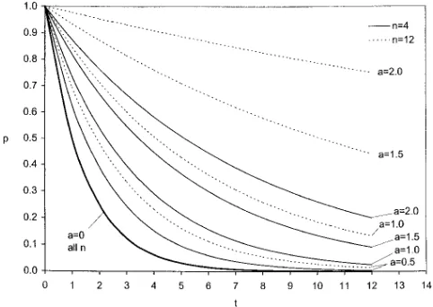
segregation at other loci in a way that the accuracy of Some examples using Equation 3 are given in Figure
1. The main point is that the differences between the probability of continued segregation of a QTL of large effect and a QTL of small effect becomes wider as more generations of backcrossing are undertaken and more intense selection is practiced. Of course, if backcrosssing is continued too long, even those of very large effect are lost. In principle, there is some intermediate opti-mum time for discriminating among QTL of specified effects, if such can be defined.
Since a number of independent replicate lines can be kept, it is useful to reconsider these results in terms of the distribution of the number of lines in which a QTL of specified effect would be segregating. If M lines are maintained, then the expected number in which
there is segregation at generation t is MP(n,a)t. The
actual number segregating, m, has a binomial distribu-tion, but the Poisson distribution gives an adequate
ap-Figure1.—Probability that a QTL of effect a remains
segre-proximation and results are more readily generalized.
gating for t generations of backcrossing when the best
individ-Hence, we assume that m has a Poisson distribution with
ual of n is selected each generation: P(n,a)tplotted against t
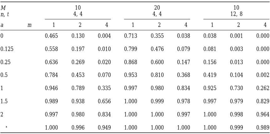
TABLE 2
Probability distribution of the number m of a total of M lines in which a QTL of effect a SD units remains segregating for t generations with selection of the best one from n each generation
10 20 10
M
4, 4 4, 4 12, 8
n, t
a m $1 $2 $4 $1 $2 $4 $1 $2 $4
0 0.465 0.130 0.004 0.713 0.355 0.038 0.038 0.001 0.000
0.125 0.558 0.197 0.010 0.799 0.476 0.079 0.081 0.003 0.000
0.25 0.636 0.269 0.020 0.868 0.600 0.147 0.156 0.013 0.000
0.5 0.784 0.453 0.070 0.953 0.810 0.368 0.419 0.104 0.002
1 0.946 0.789 0.335 0.997 0.980 0.834 0.925 0.730 0.262
1.5 0.989 0.938 0.656 1.000 0.999 0.978 0.997 0.979 0.829
2 0.997 0.980 0.834 1.000 1.000 0.997 1.000 0.998 0.964
→∞ 1.000 0.996 0.949 1.000 1.000 1.000 1.000 0.999 0.989
2, for experiments in which 10 or 20 lines are main- and 0.292, respectively. It seems that the quantitative
tained. For example, if 10 lines are maintained with differences are rather small, and that the simple
calcula-selection of one from n 5 4 for t 5 4 generations, a tions are adequate unless the segregation variance, VA,
QTL with effect of 0.25 SD has a probability of,2% of is much larger than VE(i.e., heritability in the F2
consid-remaining segregating in four or more lines, whereas a erably in excess of one-half) and if, because of the
selec-QTL with effect of 1.5 SD or more, has a,1% chance tion, it declines much more slowly than one-half per
of being lost from all 10 lines and a 66% chance of generation, i.e., there are other QTL of large effect or
remaining segregating in four or more lines. linked in coupling phase.
Correction for background genetic variation: With Two loci:The usefulness of the method depends not
segregation at other loci than that being analyzed, there only on keeping QTL of large effect segregating, but
will be additional variation within families, particularly also on losing those of small or negative effect that may
in early generations. With additive genes and genetic be maintained by linkage to a QTL of large effect. Let
variation VA caused by background genetic variation in us consider a model where there are two additive (i.e.,
the F2, and assuming for simplicity that the background nonepistatic) QTL, A1 and A2, on the same
chromo-variation is caused by very many unlinked loci, each of some, with effects a1and a2within family standard
devia-very small effect, there will be VA/2 in the first backcross tions, respectively. The recombination fraction is r
be-and VA/2tin the tth backcross. There will also be variance tween the loci. In any generation where the backcross
a2VE/4 caused by the QTL under consideration in the
parent is a double heterozygote, A1A2/A91A92, there are
first backcross, which with additive gene action implies four possible offspring genotypes selected in the next
a2VE/2 in the F2, where VEis the within-family
environ-generation: the double heterozygote with both A1and
mental variance. Consider a simple case, where VA5VE A2 present, i.e., A1A2/A91A92 with probability P12(n,a1,a2), and a51, so the total genetic variance in the F2would or the single heterozygote with only A1, i.e., A1A92/A91A92
be 3VE/2, and the within-family environmental plus with probability P129(n,a1,a2), or only A2, or both lost.
background genetic variance in the backcross would An extension of Equation 1 can be used. For example,
be [1 1 (1/2)t]VE. Hence, the effect of the QTL in
the probability that the double heterozygote is selected
environmental SD units would be 0.816, 0.894, 0.942, . . . is given by
in backcross generations t51, 2, 3,... For example, P(4,
P12(n,a
1,a2)5[n(12r )/2n]
#
∞
2∞[(12r )F(x1a11a2)
0.816)50.698, P(4, 0.894)50.714, and P(4, 0.942)5
1rF(x1a2)1rF(x1a1)1(12r )F(x )]n21φ(x )dx.
0.724, whereas P(4,1)5 0.735. Hence, the probability
(4)
that the QTL remains segregating to generations 1, 2,
Similar equations apply for sampling the other geno-3, and 4 is 0.697, 0.498, 0.361, and 0.26geno-3, respectively,
types, the term in (1 2 r) before the integral being
whereas the equivalent values assuming that P(4,1) is
TABLE 3
Probabilities of selection of each alternative genotype for a two-locus model with additive effects a1
between alleles A1and A91at locus 1 and a2between A2and A92at locus 2, and recombination
fraction r between the loci—selection of the best one from n
n 4 12
r A1A2 A1A29 A91A2 A91A29 A1A2 A1A92 A91A2 A91A92
a1: 0.5 a2: 0.5
0.5 0.380 0.242 0.242 0.136 0.468 0.222 0.222 0.089
0.2 0.596 0.095 0.095 0.214 0.704 0.083 0.083 0.131
0.1 0.666 0.047 0.047 0.240 0.776 0.040 0.040 0.144
0.05 0.701 0.023 0.023 0.252 0.811 0.020 0.020 0.150
0 0.735 0.000 0.000 0.265 0.845 0.000 0.000 0.155
a1: 0.75 a2: 0.25
0.5 0.377 0.305 0.183 0.135 0.456 0.319 0.139 0.086
0.2 0.594 0.120 0.072 0.214 0.697 0.122 0.052 0.129
0.1 0.665 0.060 0.036 0.239 0.772 0.060 0.026 0.143
0.05 0.700 0.030 0.018 0.252 0.808 0.030 0.013 0.149
0 0.735 0.000 0.000 0.265 0.845 0.000 0.000 0.155
a1: 1.0 a2: 0.0
0.5 0.368 0.368 0.132 0.132 0.422 0.422 0.078 0.078
0.2 0.588 0.147 0.053 0.212 0.676 0.169 0.031 0.124
0.1 0.662 0.074 0.026 0.238 0.760 0.084 0.016 0.140
0.05 0.698 0.037 0.013 0.252 0.802 0.042 0.008 0.148
0 0.735 0.000 0.000 0.265 0.845 0.000 0.000 0.155
a1: 1.5 a2:20.5
0.5 0.336 0.476 0.064 0.124 0.317 0.611 0.017 0.054
0.2 0.567 0.201 0.026 0.206 0.602 0.282 0.009 0.108
0.1 0.650 0.102 0.013 0.235 0.717 0.148 0.005 0.130
0.05 0.692 0.051 0.007 0.250 0.779 0.076 0.002 0.142
0 0.735 0.000 0.000 0.265 0.845 0.000 0.000 0.155
remains segregating, in subsequent generations its be- 0.25)50.074, compared with the exact values of 0.594,
0.120, and 0.072, respectively, in Table 3. havior in that line is described as would be for single
loci (1). The examples in Table 3 are for nonepistatic loci,
i.e., with additive effects in heterozygotes over loci.
Equa-Examples are given in Table 3 of the probabilities for
a series of examples in which the sum of the effects of tion 4 changes in a straightforward way if this is not
the case, and probabilities that one or both of the loci the two loci are the same (a11a251), but their relative
sizes differ (a15 0.5, 0.75 and 1.5). Results for a15 1 continue to segregate change correspondingly. For
ex-ample, consider the case where the double heterozygote
and a250 can be obtained from Table 1 by noting that
P12(n,1,0) 5 (1 2 r)P(n,1), where P(n,1) is given by is 1 SD superior to each single heterozygote and the
double homozygote. For complete linkage (r 50),
re-Equation 1. If linkage is loose, it is seen that the extreme
sults are therefore the same as in each example in Table
cases of equal effects (a1 5 a2) and a2 , 0 give quite
3, whereas for r50.2, P1250.6376, P1295P19250.0604, different outcomes, but as linkage becomes tight, the
and P1929 5 0.2416, and for unlinked loci (r 5 0.5), survival probability of the double heterozygote depends
P1250.4502, and P1295P1925P192950.1832, i.e., single little on the relative size of effects of the two loci.
heterozygotes are less likely to be selected than in the These probabilities can be approximated, providing
additive case. values of ia1and ia2are not too large, for example:
To consider the passage over several generations of
P12(n,a
1,a2)z(12r )[11i (a11a2)/2]/2,
each of the genotypic classes, it is necessary to include
P129(n,a
1,a2)zr [11i (a12a2)/2]/2, (5) the probabilities of the single locus segregants. We con-struct the 333 transition matrix B, for which the rows and similarly for P192(n,a1,a2). For example, with r50.2,
these approximations give values of P12(4, 0.75, 0.25) and columns identify the following states: (1) A1 and
A2, (2) A1but not A2, and (3) A2but not A1; the elements
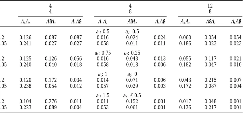
TABLE 4
Probabilities of segregation after t generations of alternative genotypes for a two-locus model with additive effects a1between alleles A1and A91at locus 1 and a2between A2and A92at locus 2, with
recombination fraction r between the loci—selection of the best one from n each generation
4 4 12
n
4 8 8
t
r A1A2 A91A2 A1A92 A1A2 A19A2 A1A92 A1A2 A91A2 A1A92
a1: 0.5 a2: 0.5
0.2 0.126 0.087 0.087 0.016 0.024 0.024 0.060 0.054 0.054
0.05 0.241 0.027 0.027 0.058 0.011 0.011 0.186 0.023 0.023
a1: 0.75 a2: 0.25
0.2 0.125 0.126 0.056 0.016 0.043 0.013 0.055 0.117 0.021
0.05 0.240 0.040 0.018 0.058 0.018 0.006 0.182 0.047 0.010
a1: 1 a2: 0
0.2 0.120 0.172 0.034 0.014 0.071 0.006 0.043 0.215 0.007
0.05 0.238 0.054 0.012 0.057 0.029 0.003 0.172 0.087 0.004
a1: 1.5 a2:20.5
0.2 0.104 0.276 0.011 0.011 0.152 0.001 0.017 0.048 0.001
0.05 0.223 0.089 0.004 0.053 0.061 0.001 0.136 0.217 0.001
bi,jspecify the transition probability from state i at gener- and are simply a special case of the two-locus analysis
given above. Let us assume that A1is the QTL and A2
ation t to state j at generation t 1 1. (Alternatively, a
4 3 4 matrix can be used, with the fourth row and is the marker, i.e., a15a and a250, with the
recombina-tion fracrecombina-tion between the loci equal to r. Then the
ele-column denoting the case where neither A1nor A2are
ments of B are given by segregating; because this is an absorbing state, the
com-putation of segration probabilities are not affected.) b
115(12r)P(n,a), b125rP(n,a), b135r[12P(n,a)], Hence, using the single locus formulas from the
preced-b225P(n,a), b3351⁄2 ing section,
where P(n,a) is given by Equation 1. An example for a marker locus is given as part of Table 3 (a151, a250). B5
1
P12(n,a
1,a2) P129(n,a1,a2) P192(n,a1,a2)
0 P(n,a1) 0
0 0 P(n,a2)
2
. (6) The probability, from Equations 7a and 7c, respectively,
that the marker remains segregating in coupling with the QTL is
Assuming the population starts in the state where both
P12(n,a,0)
t5[(12r )P(n,a)]t,
A1and A2 are segregating, from Equation 6, it can be
shown that at generation t, the probability it remains segregating without the QTL
P12(n,a
1,a2)t5bt11, (7a) is
P1(n,a
1,a2)t5b12(b11t 2bt22)/(b112b22), and (7b) P192(n,a,0)t5[r(1 2P(n,a)]{(1⁄2)t2[(12r )P(n,a)]t}/
P2(n,a
1,a2)t5b13(bt112bt33)/(b112b33). (7c) {1⁄22[(12r )P(n,a)},
For the example given in Table 3, results for segration and their sum, P12(n,a,0)t 1 P192(n,a,0)t, is the overall
probabilities for four and eight generations are given in probability the marker is retained. Because the
probabil-Table 4. Although the probability that both loci remain ities that QTL are retained for many generations are
segregating is not greatly affected by the relative magni- already small unless the QTL has an effect as large as
tude of the gene effects (and no probabilities of reten- 2 SD or so (Figure 1), it is clear that only very tightly
tion are high in this example because the total effect is linked markers are likely to be of value in QTL
detec-only a1 1 a2 5 1 and n 5 4), the QTL of smaller or tion. An illustration is given in Table 4 (a1 5 1, a2 5
negative effect has a low probability of remaining segre- 0). Hence, the marker analysis after backcrossing needs
gating alone for many generations, so the method does to be done with very closely spaced markers in a
genome-have some discriminating power. wide scan.
Marker segregation:The previous analyses have been If there are two QTL, the fate of alleles at a marker locus, say A3, depends on whether it is between or out-restricted to the fate of the QTL, but their segregation
has to be detected by means of molecular markers. The side this pair. If A3is outside the interval A1–A2, then its
TABLE 5
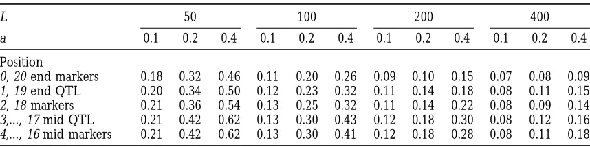
Probabilities of segregation of multiple QTL and markers, computed using Monte Carlo simulation with 500 replicates*
L 50 100 200 400
a 0.1 0.2 0.4 0.1 0.2 0.4 0.1 0.2 0.4 0.1 0.2 0.4
Position
0, 20 end markers 0.18 0.32 0.46 0.11 0.20 0.26 0.09 0.10 0.15 0.07 0.08 0.09
1, 19 end QTL 0.20 0.34 0.50 0.12 0.23 0.32 0.11 0.14 0.18 0.08 0.11 0.15
2, 18 markers 0.21 0.36 0.54 0.13 0.25 0.32 0.11 0.14 0.22 0.08 0.09 0.14
3,..., 17 mid QTL 0.21 0.42 0.62 0.13 0.30 0.43 0.12 0.18 0.30 0.08 0.12 0.16
4,..., 16 mid markers 0.21 0.42 0.62 0.13 0.30 0.41 0.12 0.18 0.28 0.08 0.11 0.18
* SE (probability estimate),2%, dependent on actual probability and map position.
A chromosome of map length LcM comprises 21 equally spaced loci, numbers 0 and 20 being at the ends. There are QTL of effect a in coupling at positions 1,3,..., 19, and markers with no effect at positions 0, 2, ...,
20. Results given are averages over the loci indicated. n54, t54.
formulas given in Equation 3. If A3lies outside the inter- chromosomes is 4 SD. In general, there will be greater
discrimination if selection is more intense and the num-val, but nearer to A2, for example, the probability that
all three loci remain segregating is given by (1 2 bers of generations are longer than the examples in
Table 5 (n5 4, t5 4). A model with very many QTL
r23)P12(n,a1,a2). If A3 lies between A1 and A2, then, for
example, the probability that all three loci remain segre- of very small effect in coupling would give similar results
to those in Table 5, as seen by the similar segregation gating is [(1 2r13)(1 2r23)/(12r12)]P12(n,a1,a2). The
matrix has to be formally extended to consider seven probabilities for QTL and markers.
Unless the chromosome is very long (L. 200) and
possible classes (all three loci, three pairs, and three
singles), but the calculations are straightforward. individual QTL are all of large effect (say a . 1), an
alternative extreme model in which there is complete
Multiple linked QTL: The preceding analysis is
con-cerned with the outcome of backcrossing when there repulsion of QTL, i.e., alternating positive and negative
effects on the trait along the chromosome with no net are only one or two QTL on the chromosome affecting
the trait under selection. An alternative model is that effect of the QTL together on the chromosome, would
behave in a very similar way to the case in which all loci the difference in performance between the recurrent
and nonrecurrent parent lines are caused by many QTL are neutral. In general, there will be greater
discrimina-tion if selecdiscrimina-tion is more intense and the numbers of of (mainly) small effect on each chromosome. Some
examples have been considered using the Monte Carlo generations are longer than the examples in Table 5
(n5 4, t5 4). simulation, with a model of a chromosome of map
length LcM and typically 21 loci simulated at equal Interspersed inter se matings: QTL of small effect,
particularly if they are partially recessive to that in the spacing, with the most distant at the ends of the
chromo-some. Ten of these loci, numbers 1 (i.e., at position recurrent parent, have a low probability of retention. It
is possible to increase the probability of QTL segrega-0.05L), 3,..., 19, were assumed to be QTL of equal effect,
and the remaining 11 loci, numbers 0, 2,..., 20, were tion by increasing the strength of the selection in
in-creasing frequency relative to that of backcrossing in assumed to be markers with no effect on the trait. The
probabilities that individual QTL remain segregating reducing frequency. One possible method, which fits
within the independent family (line) structure discussed do not differ greatly whether or not they are near the
middle or the end of the chromosome, unless the chro- here, is to intersperse a generation of inter se mating
between each generation of backcrossing, i.e., to allow mosome is of length 200 cM or more. Similarly, the
probability that individual markers remain segregating two generations of selection per generation of
back-crossing. For simplicity, it is assumed that the same fam-is little different from that of the QTL between which
they lie. Hence, only summary figures are given for the ily size is used in each case: in the backcrossing
genera-tions, the best male (or female) from n of that sex is
examples in Table 5. If the chromosome is short (L,
100), the probability that loci on it remain segregating selected; in the inter se generation, the best male from
n males recorded and the best female from n females
is quite substantial, even if the individual loci have
ef-fects of 0.4 SD or less. If it is long (L . 200), the recorded are selected and mated. The important
differ-ence from the previous analysis is that now matings can probability of continued segregation is a little higher
than for neutral genes (6% in the example of t 5 4 be made between two heterozygotes so that
homozy-gotes for the QTL of interest may then be selected for generations), even if the individual effects are as large
In the previous analysis of backcrosses alone, the spersed generation does not half the rate of loss (i.e.,
1 2 l) unless the effect of the QTL is quite large.
quantity a was used for simplicity to define the
homozy-gote–heterozygote difference; a fuller definition is now Because the time (i.e., total number of generations)
required to reduce the probability of segregation of
required, and the notation ofFalconer andMackay
(1996) is adopted, adding an asterisk to distinguish val- neutral background genes is doubled, it is moot whether
there is benefit in inserting the inter se generation. Main-ues from those above: the genotypic valMain-ues (in within
family SD units) are AA a*, AA9d*, and A9A9 2a*. Hence, taining more replicate lines or increasing the number
of individuals from each family recorded for the quanti-in the previous analysis, a5a* 1d*. If the parents of
the inter se generation are a homozygote and a heterozy- tative trait, each generation, family size may make more
efficient use of resources. Where reproductive rate lim-gote, the calculations given in Equation 1 still apply. If
the mating is between two heterozygotes, the probabili- its selection intensity, for example in mice, it might be
increased by keeping two litters from each female or ties that the individual selected for the next backcross
generation is AA, AA9, or A9A9are readily computed by by selecting only among males that have been given
multiple matings. extending the formula, as exemplified by Equation 4.
Let these probabilities be, for example, PAA(n,a*,d*). The full two-generation process can be described by a
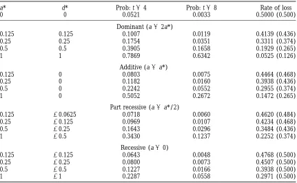
DISCUSSION
transition matrix C, in which the rows and columns
denote the genotype of the backcross parent, AA for To convey some “feel” for the results, examples of
simulated data sets are given in Table 7, in each case for the first and AA9for the second (a third row and column
could be added for the absorbing state when the back- a single chromosome of length 1 Morgan and following
eight generations of backcrossing with selection of the cross parent is A9A9):
best individual from 12 recorded. The different models
C5
1
PAA(n,a*,d*)
[P(n,a*1d*)]2PAA(n,a*,d*) simulated represent different distributions of the QTL
effects, ranging from ai 5 0.2 to 2, but with the same
total difference in effect,Riai 52, between these
chro-PAA9(n,a*,d*)
[P(n,a*1d*)]2{PAA9(n,a*,d*)12[12P(n,a*1d*)]}
2
.mosomes (as heterozygotes) from the recurrent and nonrecurrent backcross lines. The variances in the F2
In the first row of C, because the backcross parent is would differ among the models (unless there was no
AA, the mating for the inter se generation is always AA9 recombination), being largest with only one QTL
differ-3AA9, so the probabilities c11and c12refer to the selec- entiating the lines. As expected from the previous
analy-tion of AA and AA9, respectively, from among their off- ses, there is segregation at one or more of the markers
spring. In the second row, where the backcross parent in the majority of the replicate backcross lines. It is also
is the AA9 heterozygote, the probability is [P(n,a* 1 seen that the pattern differs somewhat according to the
d*)]2that both the selected male and female for the inter
number of QTL accounting for the line difference on
se mating are heterozygote, which leads immediately to this chromosome, but that many marker configurations
c21and the first term in c22. The second term in c22 is can appear for two or more quite different distributions
the product of the probabilities, 2P(n,a* 1 of QTL effects, and that identifying whether one or
d*)[12P(n,a*1d*)], that the inter se mating is between more QTL are responsible for the marker effects seen
a homozygote and heterozygote, and P(n,a*1d*), that is unlikely to be feasible from the marker distribution
a heterozygous offspring is selected from the mating. alone. As in other methods of QTL mapping, it is
diffi-In Table 6, examples are given assuming that n54 cult to distinguish between one QTL and a pair of closely
individuals are recorded per family in both the back- linked QTL (Haley and Knott 1992; Jansen 1993;
cross and inter se mating generations, for different de- Zeng1993).
grees of dominance. The value of t refers to the number Putative evidence for a QTL in the region of a marker
of backcross generations completed, and the probabili- comes from finding that the marker is present in more
ties given are that the QTL is still segregating, i.e., the replicate lines than expected by chance. If there is no
individual selected from the inter se generation is either QTL in the region, the probability that the marker
re-AA or re-AA9. For reference, to define the rate of loss after mains segregating is 1/2t, and if M lines are maintained,
a few generations, values of 12 l, wherelis the larger the probability that it is found in m of them is given
eigenvalue of C, are also given and can be compared by the Poisson distribution with parameter M/2t. For
directly with the probabilities 12 P(n,a), which equal example, with four generations of backcrossing, the
12eigenvalue for a 131 matrix), from Table 1 when probability that it is found in three or more lines is
only backcrossing with selection is practiced. ,5% (0.026, extending results of Table 2). Hence, in
The greatest benefits from the inter se mating arise, such an experiment, applying a site-by-site type I error,
of course, when the QTL of high value is recessive and further attention should be given to regions that are
therefore neutral during the selection among back- found segregating in three or more lines. In an
inter-TABLE 6
Probabilities (Prob: t ) that a QTL is retained with t of each of alternating generations of backcrossing and inter se mating, with one individual of each sex selected from n54 recorded in each case.
a* d* Prob: t54 Prob: t58 Rate of loss
0 0 0.0521 0.0033 0.5000 (0.500)
Dominant (a52a*)
0.125 0.125 0.1007 0.0119 0.4139 (0.436)
0.25 0.25 0.1754 0.0351 0.3311 (0.374)
0.5 0.5 0.3905 0.1658 0.1929 (0.265)
1 1 0.7869 0.6342 0.0525 (0.126)
Additive (a5a*)
0.125 0 0.0803 0.0075 0.4464 (0.468)
0.25 0 0.1182 0.0160 0.3938 (0.436)
0.5 0 0.2242 0.0552 0.2955 (0.374)
1 0 0.5052 0.2672 0.1472 (0.265)
Part recessive (a5a*/2)
0.125 20.0625 0.0718 0.0060 0.4620 (0.484)
0.25 20.125 0.0969 0.0107 0.4234 (0.468)
0.5 20.25 0.1643 0.0296 0.3484 (0.436)
1 20.5 0.3430 0.1237 0.2252 (0.374)
Recessive (a50)
0.125 20.125 0.0643 0.0048 0.4768 (0.500)
0.25 20.25 0.0800 0.0073 0.4507 (0.500)
0.5 20.5 0.1227 0.0166 0.3938 (0.500)
1 21 0.2287 0.0558 0.2971 (0.500)
The rate of loss of the QTL is given by 12 l, where l is the eigenvalue of the transition matrix C, and ( ) gives the rate of loss for backcrossing alone with the same QTL effects, i.e., AA a*, AA9d*, A9A9 2a*, with
effect in the backcrossing generation a5a*1d*.
remaining segregating should be considered further. 2Ri(12ri)t], a result obtained by using transition
prob-ability matrices such as B (Equation 6) or the methods This does not take into account the multiple testing
problem, which is straightforward if all markers are on of Visscher and Thompson (1995) and by ignoring
double recombinants. In any case, if the parental lines different chromosomes, or if the markers are essentially
unlinked because they are widely separated on fewer differ in mean performance and if there is evidence of
segregation variance in the initial backcross or an F2 chromosomes; the Bonferroni correction can then be
applied to give an experiment-wide error of specified of the lines, it is moot whether the genome-wide null
hypothesis of no effects is relevant. It might be more value, albeit at the risk of considerable reduction in
power. For example, taking 20 unlinked markers, one appropriate to assume an infinitesimal model (
Vis-scherandHaley1996), with the variance distributed
per mouse chromosome, the overall type I error if only
markers found segregating in four or more of 10 con- equally among and within the chromosomes: it seems
likely, however, since the net difference between the
genic backcross lines are examined further is z8%
(0.004320, from Table 2); more precisely, the probabil- two lines is therefore likely to be small around any
marker, that the probabilities of continued segregation ity that a locus remains segregating is (1/2)8, and the
probability that any of the 20 remain segregating is of each marker will be little higher than in the neutral
case unless the variance of aggregate effects among 12[12(1/2)8]2057.5%. A more sophisticated analysis
is required to find critical values when the distribution marker intervals is large.
It is possible, at least in principle, to estimate the of chromosome lengths and actual position of markers
are taken into account, but it is quite straightforward effects of a QTL located near a marker from the number
of replicate lines in which it is segregating. Considering to obtain genome-wide critical values such as those that
are used in QTL mapping from one-generation crosses first individual QTL, the expected proportion of lines
in which it is segregating is given by P(n,a)t, which can (LanderandBotstein1989), for example, by a
permu-tation test. It can be shown that for a chromosome be equated to the actual proportion m/M (this is the
maximum likelihood estimator). If there is no recombi-with k markers, the recombination fractions between
the adjacent markers being r1, r2, ..., rk21, then the proba- nation between the marker and QTL, an estimate, aˆ,
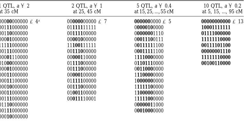
TABLE 7
Simulated examples of patterns of markers for different models of QTL distribution with the same total effect on a chromosome of length 100 cM, with 11 equally spaced markers at 0, 10, ..., 100 cM.
1 QTL, a52 2 QTL, a51 5 QTL, a50.4 10 QTL, a50.2
at 35 cM at 25, 45 cM at 15, 25, ..., 55 cM at 5, 15, ..., 95 cM
0000000000034a 0000000000037 000000000035 00000000000313
00111000000 01111111111 00000100000 10001111111
00110000000 00111100000 00000001110 01111000000
00001000000 00001000000 00011100111 11111110000
11111000000 11100111111 00111111100 00111101100
00111000000 00111000000 00011111100 00000001110
00001110000 00000110000 11110000000 11111110000
01000000000 01111000000 01101110000 00100110000
00001000000 00111000000 00110000000
00011000000 00000100000 11100000000
00011100000 01111100000 10000000000
00010000000 00111000000 11111100000
00011000000 01001100000 11000000000
00111000000 00011110001 11111000000
01110000000 00000011000
00111000000 00010000000
00010000000
aNumber of occurrences of haplotype of recurrent parent. Results for other replicates are given in the
ordered sampled. Boldface shows flanking markers for the QTL.
n5 12, t58 and M520 lines. Symbols show the marker haplotype of selected individual; 11111111111 is the marker haplotype of the nonrecurrent and 00000000000 that of the recurrent inbred parent.
evaluating Equations 1 and 3. As an approximation, so the most likely QTL position is between markers 4
and 5. Among the 18 lines segregating at markers 4 or
Equations 2 and 3 can be used together to give [(11
iaˆ/2)/2]t5m/M or aˆ5(2/i)[2(m/M)1/t21]. Because 5, the QTL (let us assume identified from phenotypes for the trait) was segregating at 17; of these 18 lines, nine the estimate is obtained from a realization of the Poisson
distribution with a small parameter value, the standard were recombinants between marker 4 (map position 30
cM) and the QTL, and five were recombinants between error of the estimate is likely to be of the same size as
the estimate itself, which can be considered as no more the QTL and marker 5 (map position 40 cM). Hence,
the maximum likelihood estimate of QTL position can than a guide. The estimate also has to be corrected for
recombination between the marker and the QTL. In be shown to be at 36.7 cM, close to its actual position
at 35 cM. The precision was achieved by typing solely principle, but beyond the scope of this paper, interval
mapping (LanderandBotstein1989) could be used 20 genotypes, but obviously, this is an extreme example
of a QTL of very large effect retained segregating over to combine the data on markers, but sampling errors
will remain large. Information on the effect of the QTL many (eight) generations. More generally, the precision
will be a function of the number of lines in which the can also be obtained directly from segregation analysis
within the backcross families at the end of the backcross- QTL remains segregating, those in which it and the
markers are lost providing none, and the number of ing phase, those retaining a QTL of large effect having
both higher mean and higher within family variance generations for which backcrossing is continued, the
effective recombination rate being 12(12r)t. There than those in which it is lost. Further precision can be
obtained by typing progeny for the marker(s) near the is, however, a trade-off because increasing the number
of generations leads to a reduction in probability of putative QTL.
A QTL can be mapped solely using the marker infor- segregation and an increase in the effective
recombina-tion rate. mation on single individuals in each family at the end
of the backcrossing phase. Consider the example in the It would be possible to obtain more information about
QTL positions and effects if the marker screening were first column of Table 7, and assume, as was actually the
model simulated, that there was only one QTL on the conducted during the backcrossing program, and this
would also enable decisions to be made as to when to chromosome, and that the lines in which the QTL was
segregating could be identified from their mean and cease backcrossing to optimize the trade-off between
recombination and loss of QTL. The records of individ-variance. In the 20 replicate lines, markers 1, 2, ..., 7
were segregating in, respectively, 1, 3, 7, 12, 11, 2, and ual animals for the quantitative trait and for each marker
maximum likelihood methods that are computationally effects and more closely map their position. Progeny testing of recombinants can be used to make this proce-feasible using Markov chain Monte Carlo methods, such
as Gibbs sampling, and have been used in an analysis dure more accurate (P. D. Keightley,personal
commu-nication). of recurrent backcross lines in which a set of different
marker regions were maintained segregating (Ranceet For precise mapping of QTL, opportunity is needed
for substantial recombination between linked QTL and
al. 1997). The simple scheme analyzed here, in which
marker information is collected only at the end, is more between them and markers. The advantage of multiple
generation schemes is that, in effect, recombination appropriate for laboratory species with short generation
intervals than for commercial animal or crop species. fractions are increased roughly in proportion to the
number of generations, and similarly, the average In such cases, it is likely to be preferable to collect
marker data each generation, and perhaps to also length of chromosome retained around a marker is
reduced in inverse proportion to the number of genera-choose individuals for backcrossing on their marker
genotype as well as on phenotype for the trait of interest. tions. The method discussed here has advantages and
disadvantages over others for QTL location. In the most This leads to more complicated design and
interpreta-tion problems than are discussed here. conventional, QTL are mapped by recording
pheno-types and marker genopheno-types in an F2or backcross of a
If only QTL on autosomes are to be identified, it
should not matter greatly whether a male or female is line cross. An additional experiment is subsequently
required to isolate these further, which can involve in-selected for the next generation of backcrossing. If,
however, QTL on the sex chromosome are to be located, trogression or retention of marked segments by
back-crossing; this contrasts with the backcrossing with selec-then females should obviously be selected in the
back-cross line; if map lengths in females are greater than tion proposed here in that it is the markers that are
identified in the backcrossing rather than the pheno-in males, there is an added benefit pheno-in dopheno-ing so. There
are other practical issues that have not been considered. types. Even so, a number of lines have to be retained
for each QTL because the precise relation between For example, there is a risk that the selected individual
in a line is infertile or that none of the required sex marker and QTL position is not known. The use of
markers, however; has the benefit that QTL of smaller are available for selection. In such cases, it may be
appro-priate to initiate many more lines than are expected to effect can be retained, and as marker and trait data
are collected throughout, information on the location be maintained, or to sacrifice the simplicities of having
completely independent backcross lines by drawing sub- accumulates during the backcrossing phase, but at the
expense of a lot of recording, compared to backcrossing lines from surviving lines to maintain numbers. The
analysis can be clearly developed further. with selection on the trait. An alternative approach is
to proceed to QTL mapping of more advanced genera-With recurrent backcrossing and selection to only
one line, QTL that are recessive in the nonrecurrent tions of the cross, for example, F3, F4,..., before
undertak-ing the QTL analysis; however, this may still require parent will be missed. Although alternating
backcross-ing and inter se matbackcross-ing alleviates this problem, net selec- backcrossing to establish congenic lines for gene
clon-ing. (Recurrent backcrossing rather than inter se mating tive pressures on recessives remain small. An alternative,
if both lines are inbred, is to practice backcrossing and is not feasible without selection because most QTL
would be lost.) A further alternative for multigeneration selection in two reciprocal sets of lines, differing in
which is used as the recurrent parent. The probability analysis is the use of selected lines and identification
of QTL, preferably replicated by changes in marker that the QTL is maintained segregating in each type of
line and over the whole set can readily be computed frequencies between high and low lines (Keightley
andBulfield1993); however, this still requires
subse-from the methods given here.
It is important to note that the method discussed in quent backcrossing if congenic lines are needed for
precise mapping and cloning.
this and other studies (e.g.,N. J. Schork, A. M. Beebe,
B. Thiel, P. St. Jean,andR. L. Coffman,unpublished The objective of this paper is not to show that the
use of recurrent backcrossing with selection with several data) on the use of recurrent backcrossing paper is
essentially a prescreening procedure for QTL detection, independent single family backcross lines is optimal in
any broad way. It is indeed clear that if more effort were not a finishing point. When the recurrent backcrossing
with selection on phenotype for the quantitative trait is expended on recording markers during the
backcross-ing phase and associatbackcross-ing them with performance of completed, and regions of the genome which the
marker analysis indicates that QTL for the trait are likely the trait, and perhaps using this information to generate
sublines on a dynamic basis, further precision could be to be present, more detailed analysis is needed; the
congenic lines, however, provide a useful starting point. obtained; the analysis of such a scheme, however, is
beyond the scope of this paper. The aim is merely to For example, further backcrossing can be practiced
while maintaining segregating-only specific short marker suggest a method with relatively low input of effort that
may lead to fairly clear identification of QTL of large intervals. Segregation within the families and QTL and
Haley, C. S.,andS. A. Knott,1992 A simple regression method that may be useful for further, more detailed analysis.
for interval mapping in line crosses. Heredity 69: 315–324.
The idea of backcrossing with selection is old indeed, Hill, W.G., 1969 On the theory of artificial selection in finite
populations. Genet. Res. Camb. 13: 143–163.
and its successful use to identify QTL for disease
resis-Houwen, R. H. J., S. Baharloo, K. Blankenship, P. Raeymaekers,
tance has been reported (Beebeet al. 1997). The only
J. Juynet al., 1994 Genome screening by searching for shared
novelty is in the use of independent sublines and the segments: mapping a gene for benign recurrent intrahepatic
cholestasis. Nature Genet. 8: 380–386.
quantification of the probabilities that QTL are
re-Jansen, R. C.,1993 Interval mapping of multiple quantitative loci. tained.N. J. Schork, A. M. Beebe, B. Thiel, P. St. Jean
Genetics 135: 205–211.
andR. L. Coffman(unpublished data) discuss methods Keightley, P. D.,andG. Bulfield,1993 Detection of quantitative
trait loci from frequency changes at marker loci under selection.
for analysis of nonindependent backcross lines with
se-Genet. Res. 62: 195–203.
lection and use of markers. Keightley, P. D., T. Hardge, L. MayandG. Bulfield,1996 A
genetic map of quantitative trait loci for body weight in the I am grateful toPhilippe Baret, Peter Keightley, Sara Knott,
mouse. Genetics 142: 227–235.
Peter Visscher, Zhao-Bang Zeng,and two anonymous referees for
Lander, E. S.,andD. Botstein,1989 Mapping Mendelian factors
helpful comments, and to the Biotechnology and Biological Sciences
underlying quantitative traits using RFLP linkage maps. Genetics Research Council for financial support. 121:185–199.
Ollivier, L., L. A. Messer, M. F. RothschildandC. Legault,1997
The use of selection experiments for detecting quantitative trait loci. Genet. Res. 69: 227–232.
Rance, K. A., S. C. HeathandP. D. Keightley,1997 Mapping LITERATURE CITED
quantitative trait loci for body weight on the X chromosome in mice. II. Analysis of congenic backcrosses. Genet. Res. 70:
Alpert, K. D.,andS. D. Tanksley,1996 High-resolution mapping
125–133. and isolation of a yeast artificial chromosome containing fw2.2:
Snell, G. D.,1958 Histocompatibility genes of the mouse. II.
Produc-a mProduc-ajor fruit weight quProduc-antitProduc-ative trProduc-ait locus in tomProduc-ato. Proc. NProduc-atl.
tion and analysis of isogenic resistant lines. J. Natl. Cancer Inst. Acad. Sci. USA 93: 15503–15507.
21:843–877.
Beebe, A. M., S. Mauze, N. J. SchorkandR. L. Coffman,1997 Serial
Tanksley, S. D.,andJ. C. Nelson,1996 Advanced backcross QTL
backcross mapping of multiple loci associated with resistance to
analysis: a method for the simultaneous discovery and transfer Leishmania major in mice. Immunity 6: 551–557.
of valuable QTLs from unadapted germplasm into elite breeding
Charlier, C., F. Farnir, P. Berzi, P. Vanmanshoven, B. Brouwers
lines. Theor. Appl. Genet. 92: 191–203.
et al., 1996 Identity-by-descent mapping of recessive traits in
Thomas, A., M. H. SkolnickandC. M. Lewis,1994 Genomic
mis-livestock: application to map the bovine syndactyly locus to chro- match scanning in pedigrees. IMA J. Math. Appl. Med. Biol. 11: mosome 15. Genome Res. 6: 580–589.
1–16.
Darvasi, A.,1997 Interval-specific congenic strains (ISCS): an
ex-Visscher, P. M.,andS. C. Haley,1996 Detection of putative
quanti-perimental design for mapping a QTL into a 1-centimorgan inter- tative trait loci in line crosses under infinitesimal genetic models. val. Mamm. Genome 8: 163–167. Theor. Appl. Genet. 93: 691–702.
De´mant, P., and A. A. M. Hart, 1986 Recombinant congenic
Visscher, P. M.,andR. Thompson,1995 Haplotype frequencies of
strains— a new tool for analyzing traits determined by more than linked loci in backcross populations derived from inbred lines. one gene. Immunogenetics 24: 416–422. Heredity 75: 644 –649.
Dietrich, W. F., J. Miller, R. Steen, M. A. Merchant,D. Damron- Wright, S.,1952 The genetics of quantitative variability, pp. 5–14 Boleset al., 1996 A comprehensive genetic map of the mouse in Quantitative Inheritance, edited byE. C. R. Reeve andC. H.
genome. Nature 380: 149–152. Waddington.Her Majesty’s Stationery Office, London, UK. Falconer, D. S.,andT. F. C. Mackay,1996 Introduction to Quantita- Zeng, Z.-B.,1993 Theoretical basis for separation of multiple linked
tive Genetics. Ed. 4, Longman, Harlow, UK. gene effects in mapping quantitative trait loci. Proc. Natl. Acad.
Guo, S. W.,1995 Proportion of genome shared identical by descent Sci. USA 90: 10972–10976.
by relatives: concept, computation and applications. Am. J. Hum.
Communicating editor:Z-B. Zeng