The Coalescent With Gene Conversion

Copyright2000 by the Genetics Society of America

The Coalescent With Gene Conversion

Carsten Wiuf* and Jotun Hein

*Department of Statistics, University of Oxford, Oxford OX1 3TG, England and†_{Institute of Biological Sciences,} University of Aarhus, 8000 Aarhus C, Denmark

Manuscript received August 4, 1999 Accepted for publication January 18, 2000

ABSTRACT

In this article we develop a coalescent model with intralocus gene conversion. The distribution of the tract length is geometric in concordance with results published in the literature. We derive a simulation scheme and deduce a number of analytical results for this coalescent with gene conversion. We compare patterns of variability in samples simulated according to the coalescent with recombination with similar patterns simulated according to the coalescent with gene conversion alone. Further, an expression for the expected number of topology shifts in a sample of present-day sequences caused by gene conversion events is derived.

U

sequences requires insight into at least three pro- gene conversion alone. In Hilliker et al. (1994) the

cesses. The first is the genealogical process describing distribution of the gene conversion tract in Drosophila

the ancestral history of a sample of alleles from a single melanogaster is estimated. They find that a geometric

locus. Kingman’s coalescent process (Kingman1982) is distribution is a good approximation of the empirical

one such process. The second is the substitution process distribution and accordingly the model is built on this

that describes how alleles mutate over time. For neutral observation.

loci the genealogical process and the substitution pro- In a subsequent article (Wiuf 2000) it is shown that

cess can be separated such that the substitution process _{to some extent the results given in this article apply}

is superimposed on the genealogical process (Tavare´ _{generally without assuming any specific form of the}

dis-1984), whereas for loci subject to selection the two pro- _{tribution of the transferred chunk. The benefit of the}

cesses cannot be separated. Finally, the last process de- _{geometric distribution is that more analytical results can}

scribes the linkage relations between adjacent loci. It _{be proven and that a specific choice of distribution}

governs how and when adjacent loci are linked or split _{(here, geometric) allows for investigation by simulation.}

on different ancestral chromosomes and requires essen- _{Two nucleotides separated by a large distance produce}

tially an understanding of mechanisms that operate at _{recombinants due to recombination events only. The}

the sequence level. _{(short) finite length of a gene conversion tract makes}

Central to many models describing the mechanisms _{the contribution from gene conversion events}

insignifi-at the sequence level is the Holliday junction (Holliday _{cant. Thus, the patterns observed in a sample of}

se-1964). When the Holliday junction is resolved the result _{quences are the result of recombination events in the}

can be of two types: (1) a gene conversion with accompa- _{history of the sample and of the substitution process}

nying exchange of flanking regions (gene conversion _{imposed. However, over small distances recombinants}

with recombination); or (2) a gene conversion alone _{can be produced by recombination events as well as}

(Carpenter 1984; Stahl 1994). In this case a short _{by gene conversion events. The observed patterns in}

tract of nucleotides is exchanged between two strands.

samples of sequence data are thus the results of three We refer to the latter case as a gene conversion and the

different processes: the gene conversion process and the former as a recombination.

recombination process, and as well as the substitution It is the aim of this article to develop a coalescent

process. model with intralocus gene conversion alone and

inves-A recombination process was incorporated into King-tigate the effects of gene conversion on various statistics

man’s coalescent model (Kingman1982; describing the

of interest in the analysis of DNA sequences. We

com-genealogical process of a sample of sequences taken pare patterns of variability in samples simulated

ac-from a population) byHudson (1983) and has

subse-cording to the coalescent with recombination with

simi-quently been investigated by a number of authors

(Hud-sonandKaplan1985;GriffithsandMarjoram1997;

andWiufandHein1997 among others).

Corresponding author: Carsten Wiuf, Department of Statistics,

Univer-We expect that the patterns of intralocus variability

sity of Oxford, 1 S. Parks Rd., Oxford, OX1 3TG, England.

E-mail: [email protected] in a model with gene conversion are different from

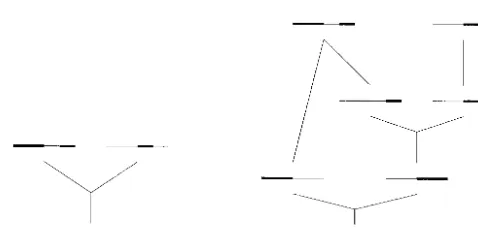
Figure1.—(A) Recombination and (B) gene conversion. If the resolution of the Holliday junc-tion results in an exchange of flanking regions we have (what here is called) a recombination event. In the top, two of the four strands involved in the Holliday junction are shown. In the bottom, time starts at present (the second generation) and goes backward. Starting with either of the two strands/sequences in the second generation, the effect of the recombination event is to create two ancestors to the sequence; the positions to the left of position S share one ancestor and the posi-tions to the right of S share another ancestor. If the Holliday junction is resolved without an exchange of flanking regions we have a gene con-version event (without recombination). In the top, two of the four strands involved in the Holli-day junction are shown. In the bottom, time starts at present (the second generation) and goes back-ward. Starting with either of the two strands/se-quences in the second generation, the effect of the gene conversion event is to create two ancestors to the sequence; the positions to the right of T and to the left of S share one ancestor and the position between S and T shares another ancestor.

those in a model with recombinants produced by recom- will only in rare cases be uniformly distributed along the

observed sequence. Again, this is in striking discrepancy bination (as defined above) only. The effect of

recombi-nation in the coalescent model is to break up the mate- with the coalescent model with recombination where

the breakpoint is uniformly distributed along the entire rial ancestral to a sequence in two parts and distribute

the parts on two different ancestors, one carrying the sequence (standard assumption; see, e.g.,Griffithsand

Marjoram1997).

ancestral material to the left of the recombination break

point, S, the other carrying the material to the right of Figure 3 shows an example of a genealogy of a sample

S (Figure 1). In contrast, gene conversion, as defined of size 2 with intralocus gene conversion.

here, breaks the material ancestral to a sequence in two This article is organized into sections. The first two

points, S and T, and distributes the material to the sections describe the coalescent model with gene

con-left of S and that to the right of T on one ancestor, and version. In the third section a simulation scheme is

the part in between S and T is on another ancestor developed similar to that ofGriffithsandMarjoram

(Figure 1). (1997) to simulate from the coalescent with

recombina-The effect of a recombination event can easily be tion; in the fourth section a number of analytical and

obtained in a model of intralocus gene conversion. If one end point falls outside the observed sequence the effect will be similar to that of a recombination event, though the probabilities of the two events might be different from each other. These probabilities depend on the rates of gene conversion and of recombination within the observed sequence. Further, they depend on the number of nucleotides observed; the higher the number the less is the chance of a gene conversion with only one end point within the observed sequence.

Similarly, the effect of a gene conversion event can be obtained by two recombination events and one

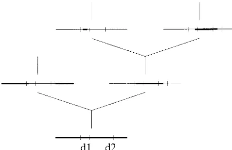
coa-Figure2.—Gene conversion vs. recombination. The

topo-lescent event (Figure 2). Again, the probabilities of

logical effect of one gene conversion event (left) can be

ob-taining the events might be very different. Especially, the

tained in a model with recombination only by two

recombina-latter series of events (given that the first recombination

tion events accompanied by a coalescence event. Assuming

event occurs) will depend strongly on the current sam- _{the rate of gene conversion events is the same as the rate of}

ple size; the higher the sample size, the lower the chance recombination events, we find that the chance of two recombi-nation events followed by a coalescence event is far smaller

that the two recombined sequences will coalesce before

than that of a gene conversion event. The former also strongly

coalescing with any other sequence in the sample.

depends on the number ancestral sequences present. Here,

Finally, the length distribution of the transferred _{for example, given that a coalescence event occurs it will result}

chunk in the gene conversion events determines the _{only in the desired distribution of ancestral material in one}

out of three possible mergings.

models of gene conversion and recombination. When proofs are omitted they can be derived from the general

results inWiuf(2000).

THE MODEL

Consider a diploid population model with effective constant (diploid) size 2N. A new generation is obtained from the present generation by sampling 2N sequences with replacement, forming random pairs of sequences, and letting a short tract of nucleotides be transferred between the sequences. The mode of transfer is de-scribed below.

Sequences are of length L ⫹ 1 nucleotides so that

there are L gaps between nucleotides. Consider one such sequence. Assume that in any generation the prob-ability of a gene conversion initiating between any two positions in the sequence is g, independently of whether gene conversions initiate elsewhere along or outside the observed sequence. Where along the sequence a gene conversion initiates is uniformly distributed among all sites. If gL is small the chance of more than one gene conversion event in one generation is negligible.

The transferred chunk of nucleotides originates from

a randomly chosen sequence in the population. InWiuf

Figure 3.—Example of a sample history with intralocus _{(2000), the length, Z, of the converted chunk can have} gene conversion. We trace the history of a sample of size 2 _{an arbitrary distribution. Here we consider the specific} back in time until all positions on the two sequences have

case where Z follows a geometric distribution with

pa-found a most recent common ancestor (MRCA). We adopt

rameter q, i.e.,

the following graphical notation: thin lines represent material nonancestral to the present-day sample; thick lines, material

P(Z|conversion)⫽ q(1⫺q)Z⫺1_{, Z} ⭓_{1. (1)}

ancestral to the sample; and crosses, material that has found

a MRCA. The first three events, 1, 2, and 3, affecting the _{That is, at least one nucleotide is transferred. It is} as-history of the sample are all gene conversion events spreading

sumed that the insertion happens to the right of the gap

the material ancestral to the sample on five sequences. From

where the conversion initiates. This model is essentially

the point of the topological structure of the tree, we cannot

distinguish events 2 and 3 from recombination events. In the equivalent to a model where the insertion happens to

first event both end points of the transferred chunk fall within _{the right of the gap with probability p and to the left} the observed sequence, whereas we cannot say whether the _{with probability 1 ⫺ p (see Wiuf 2000). The setting} other end points in events 2 and 3 fall within the observed

chosen is of mathematical convenience. If the

conver-sequence length or fall outside. All that can be said is that

sion initiates at gap S, S⫽1, 2 . . . , L (S for start), then

the other end points do not fall within material ancestral to

the present-day sample. The fourth event is a coalsecence the end point of the conversion is T⫽ S ⫹ Z (T for event whereby positions (1/2, 3/4) find a MRCA. At event 5, _{terminate). If S ⫹ Z is ⬎L, the conversion is partly} positions (3/4, 1) find a MRCA, and at event 6, positions (0, _{outside the L⫹1 observed nucleotides. The geometric} 1/2) find a MRCA. Consider the ancestral sequence A. A gene

distribution is in concordance with results inHilliker

conversion event with end points in the material not ancestral

et al. (1994) and emerges as a natural choice if the to the sample [that is outside (1/2, 3/4)] cannot be traced;

it does not affect the history. Similarly, a gene conversion probability of adding an extra nucleotide to the

trans-event in the ancestral sequence B with one or two end points _{ferred chunk does not depend on the current length.} in (1/2, 3/4) and none in ancestral material does not affect _{Later, we comment on other more realistic length} distri-the history. Only distri-the region spanned by ancestral material

butions.

need be taken into account; e.g., the span of ancestral material

Let Q⫽qL. If q is small and L is large the distribution at sequence B is 1 ⫺ 0 ⫽ 1, and the span at sequence A

is 0.75 ⫺ 0.5 ⫽ 0.25. Note that the region might include of z⫽ Z/L can be approximated with an exponential nonancestral material as in sequence B. _{distribution with parameter Q, i.e., zⵑ Exp(Q) (where}

ⵑ means “is distributed like”). Further, let G ⫽ 4gNL

be the expected number of gene conversion events per

simulated results are collected. Results obtained in the sequence per 4N generations and assume g is small

coalescent with recombination apply on several occa- and N large. The definition of G is analogous to the

sions to the gene conversion model. Finally, the last parametrization adopted for the coalescence with

re-combination (Hudson1983).

The genealogical process of a sample of n present- Denote by W_C1, the time until an event of type C1and

by W_C2the time until an event of type C2. Then we have

day sequences is studied: time starts at the present and

increases, going backward in time. Under the above W_C1 ⵑ Exp(G(1 ⫺ K(Q))/2) and W_C2 ⵑ Exp(GK(Q)/

2), such that the waiting time, WC, until a gene

conver-assumptions we find that the waiting time, WC(in units

of 2N generations), until a sequence has been created sion event of either type is WC ⫽ min(W_C1, W_C2) ⵑ

Exp(G/2). This is similar to the recombination model; by a gene conversion event that initiates within the

se-quence is approximately exponentially distributed with the waiting time to a recombination event within the

observed sequence is Exp(R/2), where R ⫽ 4rNL is

parameter G/2, i.e., WCⵑ Exp(G/2), if N is large and

gL is small. The rate of gene conversions initiating out- the rate of recombination and r is the probability of a recombination break between any two nucleotides in side the sequence but ending within the observed

se-quence must also be taken into account. This rate de- the sequence.

The end points of the tract are affected by the type, pends on the distribution of Z and is discussed in the

subsequent section. The rate of coalescence is n(n ⫺ C1or C2, of the event. The density, f␴,␶(s, t|C2), of␴and ␶conditional on C2is given by

1)/2 if there are n sequences in a sample (Kingman 1982) assuming a constant population size.

f␴,␶(s, t|C2)⫽ Q exp(⫺Q(t⫺s))K⫺1(Q),

We note that Q as well as G scale linearly in L, the

observed number of gaps between nucleotides. That is, 0⬍ s⬍t⬍1, (4)

both Q and G are doubled if the observed number of

from which the marginal densities of␴and␶easily can

gaps, L, is doubled. The expected length of the

trans-be derived. The distribution of␴(and␶) is not uniform ferred chunk in a gene conversion is 1/q (measured in

but skewed toward 0 (and 1). The density (4) is symmet-number of nucleotides). Therefore, the parameter Q is

ric so that (1⫺ ␶, 1⫺ ␴) is distributed like (␴,␶). interpreted as the sequence length measured in units

The density of (␴,␶) conditional on C2relates to that

of expected length of the transferred chunk. Similarly,

of␨conditional on C2because␨ ⫽ ␶ ⫺ ␴. We find

the parameter G is sequence length measured in

ex-pected number of gene conversion events per sequence _f

␨(z|C2)⫽ Q(1⫺ z)exp(⫺Qz)K⫺1(Q),

per 4N generations. We note that Q/G ⫽ q/(4gN) is

0⬍ z⬍1, (5)

independent of L.

where f_␨(z|C2) denotes the density of␨conditional on C2.

Finally, the density of ␴ conditional on C1 (that is,

EFFECTS OF GENE CONVERSION

␴ ⫹ ␨falls outside the observed nucleotides, ␴ ⫹ ␨ ⬎ In this section we discuss the effects of a single gene

1) is conversion event on a sequence and find the waiting

time until the sequence has been created by a gene f␴(s|C1)⫽ exp(⫺Q(1⫺ s))(1⫺ K(Q))⫺1,

conversion event.

0⬍ s⬍1. (6)

Denote by␨,␴, and␶the variables Z/L, S/L, and T/

L, respectively, where Z, S, and T are as defined in the _{If the tract falls outside the observed sequence the}

previous section. The variables ␴ and␶ take values in _{chance that ␴ is close to 1 is higher than the chance}

{1/L, 2/L, . . . , 1⫺ 1/L}債 (0, 1) and as L becomes _{that␴is close to 0. This is in concordance with (6); the}

large the distributions of␴and␶converge to continuous _{density function is increasing in s.}

distributions on (0, 1). The representation of a se- _{In Figure 4 we illustrate the above different}

distribu-quence as the continuous interval (0, 1) is commonly _{tions with q obtained from D. melanogaster data.}

used (see, e.g.,GriffithsandMarjoram1997). _{Gene conversions initiating outside the L⫹1}

nucleo-Let C denote the event that a gene conversion hap- _{tides will have a chance of terminating within the L⫹}

pens in a given sequence in a given generation. Further, _{1 observed nucleotides. Assume that the entire}

chromo-let C1 denote the event that the gene conversion falls some potentially consists of an infinite array of

se-partly outside the L ⫹ 1 observed nucleotides, that is, _{quences of length L plus the observed one of length}

S⫹Z⬎L. Similarly, let C2denote that both end points _L ⫹ _{1 and that the gene conversion model described}

are within the sequence length (lower index i indicates _{above is valid for the entire chromosome.}

that i of the two end points of the converted chunk are _{For most organisms, there is an upper bound to the}

within the L nucleotides). We find _{length of a gene conversion tract. This means that only}

a minor (finite) extension of the observed sequence P(C2|C)⫽ 1⫺

1

Q{1⫺exp(⫺Q)}⬅ K(Q) (2) should be taken into consideration and not the entire

chromosome. In the model discussed here, tract lengths

and _{can have an arbitrary size, but it can be shown that the}

probability of a tract initiating at least nL nucleotides P(C1|C)⫽1⫺P(C2|C)

away from the observed sequence and ending within the sequence, given a gene conversion event happens that

⫽ 1

because the length is exponentially distributed, and the chance that an exponential variable Exp(Q) is⬍1 is 1⫺ exp(⫺Q).

The events and Coand C1are independent. Thus, the

waiting time W_C1傼Co⫽ min(WC1, WCo) until an event of

either type C1or type Cois approximately exponentially

distributed with parameter G(1⫺K(Q)), and where the

initiation/termination point,␦, happens, is distributed with density

f␴(s|Co傼C1)⫽

1

2{exp(⫺Q(1⫺s))⫹exp(⫺Qs)}

· (1⫺K(Q))⫺1_{, 0}⬍_s⬍_1,

(9)

according to (6) and (8).

Summing up, we find that the waiting time, W, until

Figure4.—Densities of the initiation point and the length

a sequence is created by a gene conversion event is

of the gene conversion. Shown are the densities of␴

condi-exponentially distributed

tional on C1and C2, respectively, as well as the density of ␨ conditional on C2. The density of ␴given C2is found from

(4); f␴(s|C2)⫽{1⫺exp(⫺Q(1⫺s))}K⫺1(Q), 0⬍s⬍1. The _Wⵑ_Exp

冢

2

冦

Q(1⫺exp(⫺Q))

冧冣

q in D. melanogaster to beⵑ1/350 and this corresponds in this

case to an observed sequence length five times the expected _ⵑ

Exp

冢

2{2⫺K(Q)}

冣

length of a gene conversion tract or 1750 nucleotides, L⫽

Q/q.

because P(Co)⫹P(C1|C)⫹P(C2|C)⫽ 2⫺ K(Q).

Given a gene conversion occurs, the probability that both end points of the inserted chunk are within the

Basically only tracts initiating close to the observed se- observed sequence is

quence affect the sequence history in concordance with

what is expected. _{p2 ⫽}1⫺(1/Q)(1⫺exp(⫺Q))

1⫹(1/Q)(1⫺exp(⫺Q))

For each gene conversion tract initiating within the observed sequence and ending outside the observed

⫽ K(Q)

2⫺K(Q), (11)

sequence there is a similar tract initiating outside (to the left of the observed sequence), ending within the

and the probability that only one end point is within observed sequence. Because the chance of gene

conver-the observed sequence is sion events is the same along the entire chromosome,

the two events have the same probability of happening.

Let Co(o for outside) denote the event that a gene p1⫽

(2/Q)(1⫺ exp(⫺Q))

1⫹(1/Q)(1 ⫺exp(⫺Q))

conversion initiates outside the observed sequence, and terminates within. The above informal argument shows

⫽2(1⫺ K(Q))

2⫺K(Q) . (12)

that

P(Co)⫽P(C1|C) (7) Whether it is a type C_oor type C₁ event happens with

probability 1/2. The density of (␴,␶) is given by (4) (if and that the waiting time, W_Co, until a gene conversion

there are two breakpoints) and the density of the single initiating outside the observed sequence ends within

breakpoint ␴ is in the last case given by (9). In the

the observed sequence, is distributed like the waiting

example in Figure 4, Q⫽5, or five times the expected

time, W_C1, until an event of type C1; that is, WCoⵑ WC1. _{tract length, and we find p2}⫽ _{0.67 and p1}⫽_0.33.

This is a general result that applies to the models

de-The distribution in (10) is interesting for several

rea-scribed inWiuf(2000). _{sons. First, the distribution of the tract length, ␨,}

de-Further, conditional on Co, the termination point t⫽ _{pending on Q, affects the number of events and the}

T/L has density _{times between events. The parameter G(2⫺ K(Q))/2}

varies from G/2 when Q⫽∞to G when Q⫽0. Second,

f␶(t|Co)⬇

Q exp(⫺Qt)

1⫺ exp(⫺Q) for all Q⬎ 0 the number of events is higher than the

number of events in a recombination model with a

⫽ exp(⫺Qt)(1⫺K(Q))⫺1_{, 0}⬍_t⬍_{1, similar parameter (i.e., r⫽g).}

The two extreme values, Q ⫽ 0 and Q ⫽ ∞, are of

terminates when there is only one ancestral sequence

to the sample.GriffithsandMarjoram(1997)

devel-oped a similar birth and death process to handle to coalescent with recombination. Both algorithms return a genealogy in which the “true” genealogy of the sample is embedded; we keep track only of the number of sequences and the end points of gene conversions, not which parts of the sequences that are ancestral to the sample. Gene conversions can happen outside the an-cestral material to a sequence, thereby creating an “empty” sequence, i.e., a sequence with no material an-cestral to the sample (cf. Figure 2).

Consider a fixed point,␹, along the sequences. The

tree, T(␹), that describes the sequences at ␹ can be

found by starting at the present sequences and going back in time. When a gene conversion node is

encoun-Figure5.—The simulation scheme. Define G˜_⫽G(1⫹(1⫺

tered, the branch that describes the segment containing

exp(⫺Q))/Q)⫽G(2⫺K(Q)), and let k denote the number

of sequences ancestral to the sample of size n at a given time ␹ is followed. Assume that the gene conversion leaves

in the past. Further, let Ui, iⱖ1, and Vj, jⱖ1, be series of only one end point, s, in the sequence. If s⬍ ␹, then uniform variables on (0, 1). The exponential variable Wi is _{the branch describing the fate of the left part of the} the time between event i⫺ 1 and i in the samples history.

sequences is to be followed and vice versa and similarly,

Events are either coalescence or gene conversions, and if a

if the gene conversion leaves two end points. The tree

gene conversion occurs we distinguish between two types

ac-cording to the number of end points within the observed T(␹) is distributed like the coalescent process since one

sequence. With probability p1 there is one end point only, point cannot be subject to gene conversion.

otherwise two. The index i counts the number of events and _{Mutations can be superimposed on the genealogy if}

j the number of gene conversions. That is, i⫺j is the number

all alleles are selectively neutral. Assuming mutations

of coalescence events. The algorithm stops the first time there

arrive according to a Poisson process, the number of

is one ancestor to the sample.

mutations on the total genealogy is Poisson with parame-ter␪B/2, where B is the total branch length of the entire

genealogy, ␪ ⫽ 4Nu is the scaled mutation rate, and

interest. If Q⫽0 we find that WⵑExp(G), and a gene _{u is the probability of a mutation in a sequence per}

conversion will leave just one breakpoint within the _generation.

sequence. Where the break occurs will be uniformly _{The coalescent with gene conversion can be}

com-distributed along the sequence. Thus, the coalescent _{bined with the coalescent with recombination. The}

ge-with gene conversion resembles the coalescent ge-with re- _{nealogy of a sample of sequences is constructed similarly}

combination, but the rate of gene conversions is twice _{to the scheme above, waiting for three different events}

the rate of recombinations (assuming the probability of _{to occur: coalescence, recombinations, and gene}

con-a recombincon-ation between con-any two nucleotides is g). _versions.

If Q⫽ ∞we find that WⵑExp(G/2) and that both

end points of a gene conversion will be within the

se-RESULTS

quence. As Q goes toward infinity,␴will be uniformly

distributed along the sequence, and ␶≈␴, that is,␨≈ _{As noted previously, Q0⫽Q/G⫽q/(4gN) is}

indepen-0. In the limit Q⫽ ∞, a gene conversion will just leave _{dent of L. The parameters (Q0, G) are more natural}

a spot on the sequence, leaving the sequence the way _{parameters than (Q, G); G represents the length of the}

it is. Thus, the coalescent with gene conversion will _{sequence in units of gene conversion events per}

se-be indistinguishable from the pure coalescent process. _{quence per 4N generations and Q0is a parameter}

depen-Each time a conversion happens, it cannot be seen, and _{dent on the effective size of the population and}

parame-only coalescent events affect the history of a sample. _{ters intrinsic to the biological system. In contrast (Q,}

G) are both parameters representing sequence length, but in different units.

MODEL SIMULATIONS

In the following, results are given in terms of (Q0, G)

to facilitate comparisons between samples of different Assume n sequences are sampled from a present-day

population. The genealogy of the sample subject to gene lengths but with the same Q0. If we consider Q0 fixed

and G a variable, results (and plots) can be converted conversion as described in the previous section can be

simulated according to the scheme in Figure 5. between models with different g’s but equal Q0through

a linear scaling of sequence length. The algorithm is formulated as a birth and death

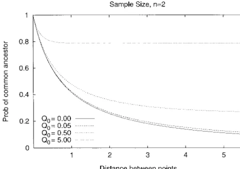
Figure6.—Probability that two positions share an ancestor,

Figure7.—Simulated values of the time until all positions

n⫽2. Shown is equation 15 for different values of Q0.

Se-have found a MRCA in a sample of size n⫽2. The expected quence length is in expected number of gene conversions per

value 2(1⫺1/n) of the time to a MRCA in a single position sequence per 4N generations. Using estimates inHillikeret

is subtracted. The curves increase with increasing values of

al. (1994), we find Q0⫽0.05 in D. melanogaster (g⫽3⫻10⫺8,

Q0. This is in agreement with the fact that the expected number q⫽3⫻10⫺3_{, and 2N⫽10}6_{). The curve for Q}

0⫽0.05 flattens

of gene conversions also increases with increasing Q0 (see out approximately at 0.027 for G⬎40 in which case Q⬎2,

Figure 9). The D. melanogaster curve, Q0⫽0.05, follows Q0⫽ or twice the expected length of a gene conversion tract. The

0 very closely (not shown). A total of 10,000 simulations were case Q0⫽0 corresponds to a model with recombination only

performed for each value of Q0. at rate 2G.

nants are produced by recombination is only G (assum-number of events per sequence per 4N generations, we

ing r⫽ g), and this is half the rate at which

recombi-find that the scaled length␨⬘ ⫽ ␨G of a tract is

nants are produced by gene conversion events. Thus,

f␨⬘(z)⫽Q0exp(⫺zQ0), z ⬎0 (13) gene conversion events might contribute significantly

to linkage disequilibrium over small distances (see also [according to (1)]; that is, exponential with parameter

Wiuf 1999). For example, according to Andolfatto

Q0⫽q/(4Ng). The waiting time, W, until a sequence is

andNordborg (1997), g⫽ 3r in D. melanogaster and created by a gene conversion event is in this formulation

the rate of gene conversions is thus sixfold that of recom-given by

bination over small distances.

Applying results in Griffiths (1991), we find for

Wⵑ Exp

冢

2 ⫹

1 2Q0

(1⫺ exp(⫺Q0G))

冣

n⫽2,

P(T2(␹1)⫽T2(␹2))⫽ Cov(T2(␹1), T2(␹2))

[from (10)]. The probabilities of the different types of gene conversion events are given by (11) and (12) with

⫽ 18⫹rG

18⫹13rG⫹ r2G

, (15)

Q replaced by Q0G. A similar remark applies to the

densities of the end points␴and␶.

In the following, we consider a sample of size n taken where Cov denotes the covariance between variables.

from the population at the present time. First, we focus We note that the expression in (15) obtains its minimum

on correlations between trees. Consider two positions, when G⫽∞, in which case rG⫽2/Q0. Thus the

covari-␹1 and ␹2, in a sample of n sequences at distance G. ance is strictly positive for all values of G and converges

We are interested in the trees, Tn(␹1) and Tn(␹2), that toward a nonzero constant as G→∞. We have

describe the sequences at␹1and␹2. Only events of type

C1 and Co in between positions ␹1 and ␹2 affect the P(T2(␹1)⫽ T2(␹2)) ⭓

(9Q0⫹1)Q0

9Q2

0 ⫹13Q0⫹ 2

. (16)

relation between the two trees. Events of type C2 in

between the positions cannot be traced. The rate, rG/2, The probability P(T₂(␹₁)⫽T₂(␹₂)) for n⫽2 is plotted

by which events of type C1 and Co happen is, per se- in Figure 6. The tree height, T_n⫽max{T_n(␹)|␹}, until

quence, _{all positions in the sample have found a most recent}

common ancestor is plotted in Figure 7 for n⫽2. For

rG⫽ 2

1 Q0

(1⫺ exp(⫺Q0G)); Q₀ ⫽ 0.05 and G⫽ 5 we find Q ⫽ 0.25, which

corre-sponds toⵑ100 nucleotides in D. melanogaster (see

Fig-ures 4 and 6). In this case the chance that two positions cf. (10) and (12).

For small values of G we find rG ≈ 2G. This is of separated at distance 5 share a most recent common

ancestor (MRCA) isⵑ0.10 if sample size is 2.

recombi-Figure8.—Number of gene conversion events. The num-ber of gene conversion events affecting the history cannot be

Figure 9.—Expected value of Gn. Sequence length is in counted by chopping up the sequence into small sections, di,

expected number of gene conversions per sequence per 4N

i⫽1, 2, . . . , counting the number, ci, in each section and

generations. As sequence length increases the expected num-then summing over i,Rici. Knowing that one end point of a

ber of gene conversions becomes effectively linear. The sample gene conversion is in section didoes not provide information

size is 10 and 10,000 simulations were performed for each whether or not the other end point is within ancestral material.

value of Q0. In the example, c1⫽2, c2⫽1, and c1⫹c2⫽3, but only two

events affect the history. Each breakpoint occurs twice in the drawing.

E[Sn]⬇2

冦

兺

i⫽1

1

i ⫺2.14

冧

Also of interest are the numbers of different types of

The proof is similar to that of Hudson and Kaplan

gene conversion events. We discuss two such numbers.

(1985; seeWiufet al. 1999 for the approximation). The

The first is the number of gene conversion events

affect-difference is the factor 2 in front, which comes from ing the history of the sample. Denote this number by

the fact that rG⬇2G for small G and not rG⫽G as with

Gn. The second is the number of gene conversion end

recombination. Again, this can result in a considerable points that make the topology change. Call this number

difference in the number of topology shifts seen in Sn. This number relates to the possibilities of detecting

models with recombination vs. gene conversion. gene conversion events in the sample history. Under an

Consider position 0 in the sequences and let Bnbe

infinite-sites mutation model (Watterson 1975) with _{the total length of the coalescent tree in position 0.}

a mutation rate very high compared to that of gene

Wiuf and Hein (1999) consider the coalescent with

conversions, G, all shifts in topologies can be detected _{recombination and discuss the sequence length,⌳}

n,

con-from sequence polymorphisms (Hudson and Kaplan _{ditional on B}

n, from position 0 until the first

recombina-1985). Also, these are the only events that can be de- _{tion point affecting the history of the sample. They find}

tected (under the infinite-sites model). _that

It is not possible to find the expectation of Gn

analyti-P(⌳n⬎x|Bn⫽b)⫽exp(⫺bx/2), x⬎0, (18)

cally. The reason for this is the following. The

expecta-tion of Gnis not linear in G because a gene conversion _{where sequence length is measured in units of expected}

with both end points in ancestral material is only _{number of recombination events per sequence per 4N}

counted once. Knowing that a gene conversion has one _{generations. Sequences are here potentially infinitely}

end point within ancestral material in a small sequence _long.

interval does not reveal if the other end point also is _{Here, we give the analogous result for the coalescent}

within ancestral material. Thus, information about gene _{model with gene conversion. The situation differs in}

conversion end points in a small sequence interval does _{the sense that we wait for either a gene conversion}

not provide information whether the points count in initiating to the right of position 0 [analogous to (18)]

Gn (Figure 8). In the coalescent with recombination, or a gene conversion initiating to the left of position 0

the expected number of recombination events can easily but ending to the right of 0. The proof is given in the

be found because the number is linear in R (Hudson appendix. The distribution of the length,⌳n, until the

andKaplan 1985). The expected value of Gn is simu- first point affecting the history of the sample,

condi-lated for different values of G and Q0 and plotted in tional on Bn, is

Figure 9. Asymptotically, the expectation of Gnis linear.

P(⌳n⬎ x|Bn⫽ b)⫽ exp{(e⫺Q0x⫺1)b/(2Q0)⫺bx/2},

The expected number of events causing a topology

Similarly, the distribution of⌳ncan be found (see

ap-pendix) and is given by

P (⌳n⬎ x)⫽

兿

i⫽1

i

i⫹ x⫹(1 ⫺exp(⫺xQ0))/Q0

. (20)

If n⫽2 we find that the expectation of ⌳nis infinite;

that is, in general the sequence length until the first gene conversion event is large. For n⬎2 the expectation is finite.

DISCUSSION

We developed a coalescent model with gene conver-sion assuming a diploid population of constant size, N.

It takes two parameters as input (along with the sample _{Figure10.—Simulated probabilities that two positions do}

size). The first is the product G⫽4NLg, where g is the _{not share the same topology for various values of Q}

0. Sequence

probability that a gene conversion tract initiates in a length is in expected number of gene conversions per

se-quence per 4N generations. Consider again D. melanogaster.

fixed position, and the second parameter is Q⫽ qL,

The curve Q0⫽0.95 follows Q0⫽0 very closely and the chance

where q is the probability that the next nucleotide is

that two points at distance 1 have different topologies is⬎70%.

within the tract given that the former is within the tract. _{This corresponds to a distance of 5% the length of the}

ex-An easy simulation scheme was developed. This scheme _{pected tract length or 0.05⫻ 350≈ 20 nucleotides. Sample}

could be modified, in accordance withGriffiths and size is 10 and 20,000 simulations were performed for each

value of Q0.

Tavare´(1994), to allow for fluctuation in the popula-tion size with time.

We derived a number of results related to the

correla-nisms operating on the molecular level in patterns of tion of trees in different positions and to the probability

variability obtained in a sample of sequences. An indica-that two given positions share a common ancestor.

tor of gene conversion could be the following. Define an These tend to be highly different from similar quantities

informative site to be a site where at least two different obtained in the coalescent with recombination. The

covariance between trees relating two distinct positions nucleotides are present in at least two sequences each.

does not tend to zero with increasing distance between Further, say a pair of sites is compatible if there exists a

the positions, but is bounded by a positive constant. topology explaining the sites with the minimum possible

Thus, it is expected that the trees in the two distinct number of substitution events. Now, assume three

infor-positions are more likely to share the same topology mative sites are given. If the first and last sites are

com-only in a model of gene conversion than in a model of patible, and the two remaining pairs involving the

mid-recombination with similar rate. Figure 10 confirms this. dle site are both incompatible, we would take this as

As Q0⫽Q/G increases, the probability,␲, of common evidence of a gene conversion event. In a pure

recombi-topology in two distinct positions decreases and for fixed nation model, given the middle site is incompatible with

value of Q0,␲converges (as function of distance) to a both other sites, we would expect that the first and the

level distinct from 0 and 1. Low values of Q0 have a last sites are also incompatible. We have simulated how

similar effect to that of recombination. often under ideal circumstances this is likely to happen.

We should note in passing that given a gene conver- It is assumed that the topology can be accurately

con-sion end point is in position ␹, the probability, p, of _{structed for each column in the sequence alignment.}

detecting that the gene conversion has occurred from _{This is, for example, the case in an infinite-sites model}

incompatibilities in the sequence alignment is very low _{with very high mutation rate. Table 1 shows simulation}

and slowly increases with sample size. Hudson and _{results for various values of Q0and G.}

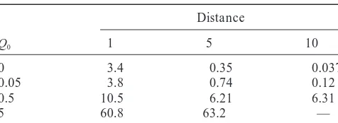
Kaplan (1985) and C. Wiuf, T. Christensen and J. _{Denote the positions 1, 2, and 3. Positions 1 and 3}

Hein(unpublished results) found _{are fixed whereas 3 is uniformly distributed between 1}

and 3. The findings in the table can be explained as

pⱕ1⫺ 2.14

log(n) follows. Assume Q0⫽0. If 1 and 2 do not share topology

and similarly for 2 and 3, this requires at least two recom-bination events. As the distance between 1 and 3 in-for large sample sizes, n; e.g., if n⫽1000, pⱕ0.69. The

creases, the chance of more recombination events

be-proof is similar to that ofHudsonandKaplan (1985)

fore the MRCAs to positions 1 and 3 increases; thus the and relates to the expected number of topology shifts

chance that 1 and 3 share the same topology decreases.

[seeHudson andKaplan 1985 and formula (17)].

TABLE 1 It would be advantageous to build a model of gene conversions and recombination more directly on a mo-Distance between 1 and 3

lecular model of these phenomena. This will be pursued in greater depth elsewhere, but the basic issues involved

Distance

are shortly sketched here.

Q0 1 5 10 _{Central to most models of gene}

conversion/recombi-nation is the Holliday junction (Holliday 1964).

Al-0 3.4 0.35 0.037

0.05 3.8 0.74 0.12 though the original Holliday model has since been

su-0.5 10.5 6.21 6.31 _{perceded by more complicated models, such as the}

5 60.8 63.2 — _{single strand invasion model (MeselsonandRadding}

1975) and the double-chain-break repair model

(Res-Shown are simulated values of the probability in percentage

that two positions, 1 and 3, share the same topology given nick 1976), the Holliday model would be still be the

positions 1 and 2, and 2 and 3 do not share topology. Position _{natural starting point for modeling gene conversion} 2 is uniformly distributed between 1 and 3. A total of 20,000 _{from a population genetical viewpoint. Issues in the} simulations were performed for each entry. The value for Q0⫽

Holliday model would also be central in the more

com-5 and distance 10 not found due to computational difficulties.

plicated models. In the Holliday model the following three problems would be of central importance.

small compared to 1/Q0(expected tract length), most

1. The movement of the Holliday junction and its con-events will be of type C1and Co. A similar pattern to that

sequences. If the movement is controlled by a ran-for Q0⫽0 is thus expected. As the distance increases, the

dom walk that is stopped at a fixed time, the length rate by which 1 and 3 are separated becomes almost

of the gene conversion would be close to a symmetric constant (rG⫽2{1⫺exp(⫺Q0G)}/Q0) and if (1, 2) and

binominal distribution moved so its mean is zero. (2, 3) do not share topologies it is most likely caused

Since the movement of the Holliday junction along by a gene conversion event with both end points within

nonidentical sequences will create heteroduplexes 1 and 3. Thus we will accept more cases where 1 and 3

that are energetically unfavorable to homoduplexes, share topology.

it could be expected that there would be a

sequence-Now fix the distance between the positions. As Q0

dependent centralizing drift in this random walk. increases, the number of C2events increases relative to

Since the energetic costs of mismatches are

approxi-C1and Coevents (Equations 11 and 12) and again if (1,

mately known, this distribution could be calculated. 2) and (2, 3) do not share topologies it is most likely

The length of gene conversions would then be se-caused by a gene conversion event that removes a region

quence dependent. This would be a complication around position 2. Again, we expect more cases where

when incorporating it into the coalescent that takes 1 and 3 share topology.

a view from the present toward the past. The pattern observed in Table 1 is obtained under

2. How is the heteroduplex corrected? Two extremes ideal circumstances. In practice, the topology relating a

can be imagined. The heteroduplex is resolved when set of sequences in a given position can be reconstructed

the DNA is duplicated or one single strand is made from the nucleotide pattern in that position in rare

the master copy and the other single strand is cor-cases only. Under an infinite-sites model with low

muta-rected so it matches to this master strand. From the tion rate, the chance that 1 and 3 can be explained by

point of view of redistributing ancestral material, this the same topology is higher than the value given in

is simple as the region within the gene conversion Table 1. Similarly, recurrent substitutions have the same

will choose one ancestor. The other possibility, that effect, but in both cases the overall pattern in Table 1

mismatches are corrected independently one by one, is retained. These results suggest that in a pure

recombi-has more drastic consequences for the distribution nation model we will see many more pairs of

incompati-of ancestral material as each correction will be inde-ble sites than in a model with pure gene conversion

pendent choices of parents. Within the region of (assuming the rate of recombination is similar to the

the gene conversion, different positions can have rate of gene conversion). On the other hand we expect

different ancestors. This would also have drastic con-many more topology shifts under a gene conversion

sequences for the phylogenetic relationships among model, so that we must return, moving along the

se-the sequences as one moves along se-the sequences, as quences, to previously visited topologies more often

even arbitrarily close positions could be related by than under a recombination model. Also, the results in

different phylogenies. Table 1 imply that recombination can be distinguished

3. The Holliday structure can be resolved in two ways, from gene conversion by the spatial arrangement of

one leading to a gene conversion, but no recombina-incompatible pairs, simply by estimating the probability

tion, and the other leading to a gene conversion and in Table 1 from data. If recombination is not present

a recombination. What are the probabilities of gene we will expect this probability to be significantly

biologi-sion is, M. Nordborg for commenting on an early verbiologi-sion of the

cal systems have gene conversion but no

recombina-manuscript, and M. Schierup for various suggestions that improved

tion. In modeling the consequences, it would be

nat-the manuscript considerably. We thank A. Mikkelsen for

implement-ural to make this probability a single parameter in _{ing the model and performing the simulations used in the article.}

the model. C.W. was supported by grant Biotechnology and Biological Sciences

Research Council 43/MMI09788 and by the Carlsberg Foundation,

Later models, especially Meselson and Radding _{Denmark. Part of this work was carried out while the authors visited}

(1975) and the double exchange model (Resnick the Isaac Newton Institute, University of Cambridge.

1976), are more complicated and will slightly change the picture. From a population genetical viewpoint, all

LITERATURE CITED

that matters in these different models is how the

ances-tral material is redistributed when viewed from the pres- Andolfatto, P.,andM. Nordborg,1997 The effect of gene conver-sion on intralocus associations. Genetics 148: 1397–1399.

ent toward the past. The Meselson-Radding model

Carpenter, A. T. C.,1984 Meiotic roles of crossing-over and of

would have a very short region with a one-directional _{gene conversion. Cold Spring Harbor Symp. Quant. Biol. 49:}

gene conversion added relative to the pure Holliday 23–29.

Griffiths, R. C.,1991 The two-locus ancestral graph, pp. 100–117

model, due to the strand invasion. Since this region is

in Selected Proceedings of the Symposium of Applied Probability, Sheffield

expected to be short relative to the length of the migra- _{1989, IMS Lecture Notes-Monograph Series, 18, edited byI. V. Basawa}

tion of the Holliday structure, the Meselson-Radding andR. L. Taylor.Hayward, CA.

Griffiths, R. C.,andP. Marjoram,1997 An ancestral

recombina-model is expected to be very similar to the pure Holliday

tion graph, pp. 257–270 in Progress in Population Genetics and

model. The double-chain-break repair model would _{Human Evolution, IMA Volumes in Mathematics and Its Applications,}

have two strand invasions and also two Holliday junc- 87, editedP. DonnellyandS. Tavare´.Springer-Verlag, Berlin.

Griffiths, R. C.,andS. Tavare´,1994 Sampling theory for neutral

tions that could undergo a random walk relative to each

alleles in a varying environment. Philos. Trans. R. Soc. Lond.

other. The double-chain-break repair model probably _{Ser. B 344: 403–410.}

has greater consequences for the distribution of ances- Hilliker, A. J., G. Harauz, A. G. Reuame, M. Gray, S. H. Clarket al., 1994 Meiotic gene conversion tract length distribution

tral material than the Meselson-Radding model, but that

within the rosy locus of Drosophila melanogaster. Genetics 137:

remains to be explored. _1019–1026.

Since it is not well known how different recombina- Holliday, R.,1964 A mechanism for gene conversion in fungi.

Genet. Res. 5: 282–287.

tion mechanisms are phylogenetically distributed, it

Hudson, R. R.,1983 Properties of the neutral allele model with

would be interesting to know if it was ever possible _{intragenic recombination. Theor. Popul. Biol. 23: 183–201.}

to distinguish the underlying mechanism from pure Hudson, R. R.,andN. Kaplan,1985 Statistical properties of the

number of recombination events in the history of DNA sequences.

population data. It would here be natural to formulate

Genetics 111: 147–164.

what was expected in terms of different sets of incompat- _{Kingman, J. F. C.,1982 The coalescent. Stoch. Process. Appl. 13:}

ibilities. For instance, if three informative sites were 235–248.

Meselson, M. S.,andC. M. Radding,1975 A general model for

given, and the first and last sites were compatible, but

genetic recombination. Proc. Natl. Acad. Sci. USA 41: 215–220.

the two remaining pairs involving the middle site were _{Resnick, M. A.,1976 The repair of double-strand breaks in DNAs:}

incompatible, this would be taken as an indicator of a a model involving recombination. J. Theor. Biol. 59: 97–106.

Stahl, F. W.,1994 The Holliday junction on its thirtieth anniversary.

gene conversion. If more informative sites were found

Genetics 138: 241–246.

close to the middle position, these would be expected _{Tavare´, S.,1984 Line-of-descent and genealogical processes, and}

to have different kinds of compatibilities dependent on their applications in population genetics models. Theor. Popul.

Biol. 26: 119–164.

which kind of repair mechanism was operating on the

Watterson, G. A.,1975 On the number of segregating sites in

heteroduplex. _{genetical models without recombination. Theor. Popul. Biol. 7:}

Whether or not different recombination/gene con- 256–276.

Wiuf, C.,2000 A coalescent approach to gene conversion. Theor.

version models are distinguishable by population

se-Popul. Biol. (in press).

quence data depends on the frequency of configura- _{Wiuf, C.,andJ. Hein,1997 On the number of ancestors to a DNA}

tions of segregating nucleotides in the population that sequence. Genetics 147: 1459–1468.

Wiuf, C.,andJ. Hein,1999 Recombination as a point process along

would result in different products when recombined

sequences. Theor. Popul. Biol. 55: 248–259.

under different models. A functional geneticist would

Communicating editor:A. G. Clark design the necessary configurations of nucleotides and

set up the adequate crosses. In population genetics this would have to occur by chance. It is unlikely that

pop-ulation sequence data can compete with designed ex- _{APPENDIX: PROOF OF FORMULAS (19) AND (20)}

periments in this respect, but this does not imply that

Wiuf andHein(1999) consider the coalescent with

different mechanisms of recombination will not have

recombination and discuss the sequence length,⌳n,

con-consequences for the expected patterns of variation in

ditional on the total branch length, Bn, from position

population sequence data; such data are becoming

avail-0 until the first recombination point affecting the history able from many organisms, where molecular genetical

of the sample. They find that experiments have not yet been performed.

where the sequence length is measured in units of ex- f␶(x|Co, G)⫽Q0exp(⫺Q0x) (1⫺exp(⫺Q0G))⫺1

pected number of recombinations per sequence per 4N _→

Q0exp(⫺Q0x), x⬎ 0 (A4)

generations. Sequences are here potentially infinitely

long. _{[from (8)]. Combining (A3) and (A4) we find the}

distri-Remember [see (10), (11), and (12)] _{bution of the length,⌳o, until the first point of type Co}

affecting the history of the sample,

W_CoⵑExp(G(1⫺K(Q0G))/2)

and _{P (⌳}o⬎x|Go⬎0, Bn⫽b)⫽

兺

∞

k⫽1

exp(⫺kQ0x)

1 k!

冢

b 2Q0

冣

k

W_C1傼C2ⵑExp(Q0G/2).

· exp(⫺b/(2Q0))

1⫺exp(⫺b/(2Q0))

Whenever an event of type C ⫽ C1 傼 C2 happens the

initiation point is uniform along the sequence (per

definition). Therefore, the sequence length, ⌳1,2from ⫽ exp(⫺b/(2Q0))

1⫺exp(⫺b/(2Q0)) position 0 until the first breakpoint affecting the history

of the sample is distributed like (A1) · {exp(e⫺Q0x_b/(2Q

0))⫺1}, x⬎0.

P(⌳1,2⬎x|Bn⫽b)⫽exp(⫺bx/2), x⬎0, _(A5)

(A2) _{Outside {G}

0⬎0},⌳0⫽∞.

Finally, combining (A2), (A3), and (A5) we deduce for sequences potentially infinitely long.

that⌳n⫽min (⌳o,⌳1,2) has distribution

The rate, G(1 ⫺ K(Q0G))/2, of type Coevents

con-verges to 1/(2Q0) for G → ∞. Conditional on Bn⫽ b,

P(⌳n⬎x|B⫽bn) ⫽exp{(e⫺Q0x⫺1)b/(2Q0) ⫺bx/2},

the number, Go, of Coevents in the sequences ancestral

to position 0 is thus Poisson distributed with parameter x⬎0, (A6)

b/(2Q0),

as required. The distribution of⌳ncan be found in the

following way. The event {⌳n⬎ x} is equivalent to the

P(Go⫽k|Bn⫽b)⫽

1 k!

冢

b 2Q0

冣

k

exp(⫺b/2Q0)),

event that no gene conversion events occur in a sample of sequences of length x before a MRCA is found. This

k⫽0, 1, . . . . (A3)

has probability The density, f␶(x|Co, G), of the termination point ␶G⫽

G␶(in units of sequence length) converges to an expo- _P(⌳

n⬎ x)⫽

兿

i⫽1

i

i⫹x⫹(1⫺ exp(⫺xQ0))/Q0

. (A7)