HIGHLIGHTED ARTICLE
| INVESTIGATION
The Genomic Basis for Short-Term Evolution of
Environmental Adaptation in Maize
Randall J. Wisser,*,1Zhou Fang,†,2James B. Holland,†,‡Juliana E. C. Teixeira,*,3John Dougherty,*,§ Teclemariam Weldekidan,* Natalia de Leon,** Sherry Flint-Garcia,††,‡‡Nick Lauter,§§,*** Seth C. Murray,††† Wenwei Xu,‡‡‡and Arnel Hallauer§§§ *Department of Plant and Soil Sciences, University of Delaware, Newark, Delaware 19716,†Department of Crop and Soil Sciences, North Carolina State University, Raleigh, North Carolina 27695,‡US Department of Agriculture-Agricultural Research Service, Raleigh, North Carolina 27695,§Center for Bioinformatics and Computational Biology, University of Delaware, Newark, Delaware 19714, **Department of Agronomy, University of Wisconsin, Madison, Wisconsin 53706,††US Department of Agriculture-Agricultural Research Service, Columbia, Missouri 65211,‡‡Division of Plant Sciences, University of Missouri, Columbia, Missouri 65211,§§US Department of Agriculture-Agricultural Research Service, Ames, Iowa 50011, ***Department of Plant Pathology and Microbiology, Iowa State University, Ames, Iowa 50011,†††Department of Soil and Crop Sciences, Texas A&M University, College Station, Texas 77843,‡‡‡Agricultural Research and Extension Center, Texas A&M AgriLife Research, Lubbock, Texas 79403, §§§Department of Agronomy, Iowa State University, Ames, Iowa 50011
ORCID IDs: 0000-0003-1075-0115 (R.J.W.); 0000-0002-4341-9675 (J.B.H.); 0000-0002-6862-3031 (J.E.C.T.); 0000-0001-7867-9058 (N.d.L.); 0000-0003-4156-5318 (S.F.-G.); 0000-0002-3127-8609 (N.L.); 0000-0002-2960-8226 (S.C.M.)
ABSTRACTUnderstanding the evolutionary capacity of populations to adapt to novel environments is one of the major pursuits in genetics. Moreover, for plant breeding, maladaptation is the foremost barrier to capitalizing on intraspecific variation in order to develop new breeds for future climate scenarios in agriculture. Using a unique study design, we simultaneously dissected the population and quantitative genomic basis of short-term evolution in a tropical landrace of maize that was translocated to a temperate environment and phenotypically selected for adaptation in flowering time phenology. Underlying 10 generations of directional selection, which resulted in a 26-day mean decrease in female-flowering time, 60% of the heritable variation mapped to 14% of the genome, where, overall, alleles shifted in frequency beyond the boundaries of genetic drift in the expected direction given their flowering time effects. However, clustering these non-neutral alleles based on their profiles of frequency change revealed transient shifts underpinning a transition in genotype–phenotype relationships across generations. This was distinguished by initial reductions in the frequencies of few relatively large positive effect alleles and subsequent enrichment of many rare negative effect alleles, some of which appear to represent allelic series. With these genomic shifts, the population reached an adapted state while retaining 99% of the standing molecular marker variation in the founding population. Robust selection and association mapping tests highlighted several key genes driving the phenotypic response to selection. Our results reveal the evolutionary dynamics of a finite polygenic architecture conditioning a capacity for rapid environmental adaptation in maize.
KEYWORDSrecurrent selection;flowering time; genetic diversity; plant breeding; agriculture; climate change
A
FTER 150 years of progress toward understanding evolution—sinceThe Origin of Species(Darwin 1859)— burgeoning experimental results fueled by advances in genomictechnology are shedding light on still unresolved questions about the nature of phenotypic change, including: the impact of mutation (e.g., Levyet al.2015) and standing variation (e.g., Burkeet al.2010; Joneset al.2012); the role of epistasis (e.g., Tenaillonet al.2012); and the relationship between natural and artificial selection (e.g., Chanet al.2012). A key question, especially in the face of biological invasions and climate change, is how genomes confer and constrain the capacity for organisms to adapt to new environments (Orr 2005). Ge-netic dissection of experimentally evolved populations is a tractable framework for elucidating adaptive evolution
Copyright © 2019 by the Genetics Society of America doi:https://doi.org/10.1534/genetics.119.302780
Manuscript received December 4, 2018; accepted for publication October 4, 2019; published Early Online October 15, 2019.
Available freely online through the author-supported open access option.
Supplemental material available atfigshare:https://doi.org/10.25386/genetics.9936284.
1Corresponding author: Department of Plant and Soil Sciences, University of Delaware,
531 S. College Ave., 152 Townsend Hall, Newark, DE 19716. E-mail: [email protected]
2Present address: Syngenta, Research Triangle Park, NC 27709.
since the experimenter can control selection and mating in particular environmental settings (Barrick and Lenski 2013; Schlöttereret al.2015). As a new extension to this framework, we implemented an efficient study design for dual infer-ence about the population and quantitative genomic basis of phenotypic evolution (Wisseret al. 2011). This was used to investigate the response to a decade of directional phe-notypic selection for tropical-to-temperate adaptation in maize—a model species for plant genetics and a crop of global importance.
Genomic Basis of Response to Phenotypic Selection
The rate and history of mutations, the numbers and positions of functional variants, the distribution of allele effects, and the modes of gene action are among the genetic factors that shape the response to selection and influence the maintenance of phenotypic and genetic variability (Barton and Keightley 2002).
Considering theoretical population and quantitative ge-netic expectations for the response to directional selection, alleles at one or few loci with large effects on a selected trait should rapidly change in frequency, resulting in a correspond-ing phenotypic response (Falconer and Mackay 1996). As these alleles approachfixation, genetic variance is reduced and the response diminishes. Sustained responses may be attributed to standing polygenic variation, new mutations, epistatic interactions, or heritable epigenetic effects. For polygenic traits controlled by numerous loci of small effects, modeled at the extreme of infinite loci (Bartonet al.2017; Fisher 1918), responses to selection can arise from subtle changes in allele frequencies across many loci. Consequently, allelic variation is retained and the causal-genic variance is expected to undergo negligible change. However, directional selection also creates negative disequilibrium covariance between allele effects across loci, resulting in temporary re-ductions in genetic variance for the trait under selection, a phenomenon referred to as the Bulmer effect (Bulmer 1971; Walsh and Lynch 2018). Qualitatively similar expectations arise under a so-called finite polygenic architecture where tens or more loci with allele effects of varying magnitudes are at play (Chevalet 1994; Fernandoet al.1994; Turelli and Barton 1994).
An empirical understanding about the genetics of adapta-tion has been advanced through experimental populaadapta-tion and quantitative genetic approaches (Savolainenet al.2013). The relative importance of genes with major and minor effects varies among traits, populations and species. At one extreme, relatively rapid or dramatic phenotypic changes have resulted from a few alleles at loci with large effects on traits such as
flowering behavior (Lowry and Willis 2010) and toxin resis-tance (Baxteret al.2011). In contrast, other dramatic shifts in adaptive phenotypes have been ascribed to a polygenic archi-tecture (Burkeet al.2010; Berg and Coop 2014). Drawing a clear line of distinction between the two is not straightforward and is partially confounded by differences in experimental
systems and their statistical power, but adaptation from a mixture of genes with major and minor effects have been reported (Levy et al. 2015). Moreover, “evolve-and-rese-quence”studies have exposed unforeseen outcomes in the genomic changes underlying phenotypic evolution, including unique patterns of allele frequency change and the mainte-nance of molecular genetic diversity (Burke and Long 2012), the direct causes of which are unresolved.
Phenological Adaptation in Maize
Pivotal to adaptation and productivity in crop species is synchrony between the growing season andflowering time (Jung and Müller 2009). Numerous studies have investigated the genetic architecture of natural variation inflowering time for maize using a variety of methods, including genic analy-sis, linkage and association mapping, ecogeographical genet-ics and historical genetic analysis. Emerging from this body of literature is a consensus that allele effects dispersed across a
finite polygenic architecture capture the major proportion of genotypic variation in flowering time (e.g., Chardonet al.
2004; Buckler et al.2009; Liet al.2016), and that certain
flowering time genes—Vgt1(Salviet al.2007; Ducrocqet al.
2008), ZmCCT10 (Hung et al. 2012; Yang et al. 2013),
ZmCCT9(Huanget al.2018), andZCN8(Guoet al.2018)— appear to have been instrumental to the postdomestication spread of maize from its tropical origin to many different environments. However, with one exception (Durandet al.
2015), to our knowledge, the genomic basis of this adaptive trait has not been investigated in experimentally evolved populations. This could fill gaps in knowledge about the evolution of adaptation and lay a foundation to innovate breeding methods for rapidly adapting populations to new environments.
In this study, we investigated the genomic basis of adap-tation from a distinct vantage point, where the entire period of evolution to an adapted state was captured in a single, multi-generational population—“Hallauer’s Tusón”(Teixeiraet al.
2015). Selection was initiated within an admixed founder population formed by intermating separate seed bank popu-lations of Tusón, a landrace historically adapted to lowland tropical environments (Goodman and Brown 1988). Remark-ably, 10 generations of directional phenotypic selection for early female-flowering time, with secondary selection for other traits in a temperate U.S. environment (Ames, IA; 42.03° N latitude), recapitulated the temperate-adapted state of maize achieved by early farmers; this is thought to have occurred over the course of thousands of years (Swarts
(Goodman 1998),findings from this study can guide future maize breeding for climate change and address fundamental questions about the genomic basis of environmental adapta-tion in plants.
Materials and Methods
Front matter
Unless otherwise noted, data analysis was performed usingR
(R Core Team 2016);Rpackages are cited accordingly. The following abbreviations are used: AFPC (allele frequency
pro-file cluster); BLUEs (best linear unbiased estimates); FDR (false discovery rate); FITR (frequency increment test with reference loci); GWA (genome-wide association); LD (link-age disequilibrium); SIM (simulation test statistic).
Plant material
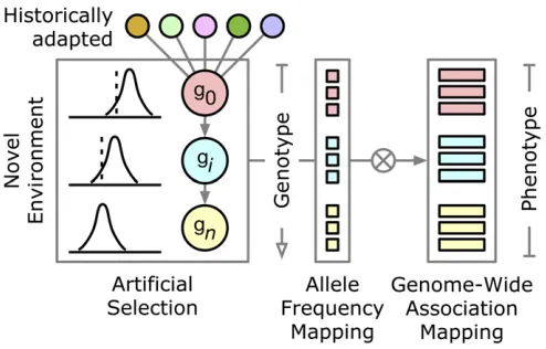
The subject of this study was Hallauer’s Tusón, a multigen-erational population of maize derived from a landrace of tropical origins that was subjected to 10 generations of phe-notypic truncation selection for early female-flowering time in a temperate environment (Ames, IA; 42.03°N latitude) (Teixeira et al.2015; Hallauer and Carena 2016). Figure 1 depicts the breeding scheme for Hallauer’s Tusón and our study design.
As described by Hallauer and Carena (2016), the base population ðg0Þ used to initiate selection was produced in Iowa by isolated, open pollination (no intentional selection) among multiple seed-bank accessions of the Tusón landrace sampled from different countries; however, the origins of some of these accessions remain unclear. It should be noted that maize is a monoecious species with female and male organs on separate parts of the same plant, such that open pollination includes the possibility of self-fertilization. Using the base population, selection ensued where 8000210;000 plants were grown in isolation and allowed to intermate at random, which again included the possibility of selfing. During
flowering, 3002500 of the earliest female-flowering individ-uals (based on their silk-emergence phenotype), secondarily selected for other traits, were tagged and later harvested. An equal number of seeds per ear were mixed to form the sub-sequent generation of8000210;000 individuals for selec-tion. This recurrent selection scheme was applied for 10 generations (from 1995 to 2004) until the population was deemed phenologically adapted by comparison with other temperate adapted maize.
Phenotype data
Previously, Teixeira et al. (2015) phenotypically evalu-ated 297 self-pollinevalu-ated ðS0:1Þ families derived from the even numbered generations of Hallauer’s Tusón (g0:n¼18;g2 :n¼56;g4:n¼56;g6:n¼56;g8:n¼56 and g10:n¼55) for two years at multiple locations in North America, including the Iowa location where Hallauer’s Tusón was originally selected. Under the design depicted in Figure 1, the present study combined the available phenotypic
data for female-flowering time measured in the selection en-vironment (Ames, IA) and a highly correlated enen-vironment (Newark, DE) with new genotype data.
Genotype data
DNA was isolated from the 297 parents (noninbred) of the S0:1 families that were evaluated phenotypically, plus an addi-tional 90 random individuals fromg0that were not pheno-typed (this was done to provide a larger sample size ofg0for more reliable genomic inference). Lyophilized leaf tissue was pulverized using a Geno/Grinder 2000 and extracted with the DNeasy 96 Plant Kit (Qiagen). Genotyping with Illumi-na’s MaizeSNP50 Beadchip (Ganal et al. 2011) was per-formed by DNA LandMarks (Québec, Canada), producing genotype data at 56;110 SNP sites with an average of 2.8% missing data per sample (min: 0.2%; max: 20.9%). Addi-tional genotype data were produced for variant sites up-stream of ZmCCT10 (Zm00001d024909) (Supplemental Material, Supplemental Methods), including a presence– ab-sence causal variant for photoperiod sensitivity (Hunget al.
2012; Yanget al.2013). See Supplemental Methods for ge-notypic data quality control (Table S1) and projection of markers onto the consensus linkage map for a maize nested association mapping population (McMullenet al.2009).
Analysis of genetic diversity
which have the lowest ascertainment bias among the Mai-zeSNP50 SNPs (Frascaroliet al.2013).
Summary statistics of genetic diversity were computed withhierfstatv. 0.04–14 (Goudet 2005) to calculateHO (av-erage observed heterozygosity within generations),H^S (av-erage expected heterozygosity within generations) andH^T9 (average expected heterozygosity for the total population), as well asF^IS(average inbreeding coefficient within genera-tions), ^FST9 (average differentiation between generations), and^FIT9(average inbreeding coefficient for the total population) according to Nei (1986)—this corresponds to the sample-level scope of inference.HardyWeinbergv. 1.5.5 (Graffelman 2015) was used to perform exact tests for Hardy–Weinberg equilibrium.
The relationship of Hallauer’s Tusón with maize more broadly was assessed using 934 samples representative of global maize germplasm for which genotype data for the same markers was available (Ganal et al. 2011). A two-dimensional projection of relationships among samples was computed usingPHATE(Potential of Heat-diffusion for Affi n-ity-based Trajectory Embedding) (Moonet al.2017) imple-mented in phateR v. 0.2.7, using default settings with a precomputed simple matching distance matrix as input for the knn.dist.method.
Results from PHATE using only Hallauer’s Tusón
sug-gested some structure was present among samples fromg0 but not other generations. Therefore,STRUCTURE(Pritchard
et al.2000) was used to examine subpopulations amongg0 samples assuming admixture and independent allele fre-quencies (Table S3; see Supplemental Methods for details). The DK method informed our selection ofK(Evannoet al.
2005). Although the exact accessions of Tusón used to form
g0 remain unclear, several were used (Hallauer and Carena 2016). Therefore, we ignored the stronger signal of DK
suggestingK= 2 and chose the next highest peak atK¼6 (Figure S1). To examine whether any one subpopulation was favored in the initial generations of selection, STRUCTURE
was also used to ascertain the g0 ancestry present in g2 samples, assuming the aforementioned subpopulation classification for individuals in g0. A paired t-test was used to test the difference between the proportion of indi-viduals per subpopulation in g0 (Table S3) and the aver-age per individual admixture proportion estimated by
STRUCTUREforg2(Table S4).
LD (Hill and Robertson 1968), measured asr2, was com-puted withgeneticsv. 1.3.8.1 (Warneset al.2013). The struc-ture of LD between chromosomes was characterized per generation using low-ascertainment biased markers with no missing data and a minimum allele count of 12 in the given generation (Table S2). The structure of LD within chromo-somes was similarly characterized, but with a larger number of markers (Table S2) and examined at different intervals of genetic distance: (0,1],(1,5],(5,10],(10,50],.50. In addi-tion,r2 was computed among generations (all samples) be-tween sequential pairs of markers per chromosome. Using these latter estimates of LD,lokern1.1.8 (Herrmann 2016)
was used to perform kernel regression of the r2 values as a function of the midpoint basepair coordinate between each pair of markers. A plot of pairwise r2 between markers flanking the ZmCCT10 associated causal site for photoperiodism was made using LDheatmap v. 0.99.2 (Shinet al.2006).
Population genetic analysis
Allele frequency mapping:Three statistical tests were used to detect markers with nonrandom patterns in allele fre-quency change across generations: (i) a customized whole genome SIM test for departures from genetic drift; (ii) the Bayenv test for robust correlations between allele frequencies and generations (Coop et al. 2010); and (iii) the FITR for robust departures from genetic drift (Nishino 2013).
A detailed description of the SIM test can be found in Supplemental Methods. Briefly, by customizing simuPOP (Peng and Kimmel 2005), a simulator was constructed to generate in silico genomes (genome-wide genotypes) for in-dividuals constituting a population that undergoes breeding according to the design for Hallauer’s Tusón (with random selection to model genetic drift) and sampling according to our study design (to account for sampling variance). The simulator used thefixedg0genotype matrix,fixed recombi-nation rates estimated from projection onto the genetic map (Supplemental Methods) and thefixed STRUCTURE matrix (Table S3) to initially generate 10;000 random in silico ge-nomes (derived based on the structuredg0sample data) from which simulated breeding ensued. At each marker across the genome, the probability of the observed sample allele fre-quency change was computed relative to the expected distri-bution created from 10;000 replicates of simulation. Marker
p-values were adjusted for multiple testing (Benjamini and Hochberg 1995), and those with a 1% FDR are referred to as SIMþmarkers, while the remaining markers are referred to as SIM2.
Bayenv 2.0 was used to identify robust correlations be-tween allele frequencies (response variable) and generations (explanatory variable). Bayenv was originally designed to test for correlations with an environmental variable; here, gener-ation numbers (standardized) were used instead. The co-variance matrix used to model the background expectation of allele frequency change was estimated from the low-ascertainment biased SNPs (Table S2). Markers with the top 1% Bayes factor values were considered robust outliers, which we refer to as Bayenþmarkers.
definable forfixed sites, yet the alleles at markers used for testing were not always observed in each generation. There-fore, alleles with an observed frequency of zero in a particular generation were set to 1=2Sg, where Sg is the number of
individuals in thegthgeneration. Markers with a 1% FDR in
at least 75% of the bootstrap sample tests are henceforth referred to as FITRþ.
Localizing footprints of selection: Chromosomal regions with a local footprint of selection (i.e., deviation from genetic drift across a segment of the genome) were delimited using chromosome-specific kernel regression functions of the 2log10ðqÞ values from the SIM test on the physical coordi-nates of markers. To obtain a definable2log10ðqÞinput value for markers where the SIM testp-value equaled 0 (where the observed data fell outside the limits of the null distribution of simulated drift), p¼0 was set to 0.00057, which was half the minimum p-value among all SIM tests. Regions along each chromosome where the kernel regression line sur-passed a threshold of2log10ðq¼0:05Þwere considered local footprints of selection, and are henceforth referred to as SIMþregions.
Characterizing features of allele frequency change:Divisive analysis of hierarchical clustering (Kaufman and Rousseeuw 1990) was performed with cluster v. 2.0.7 (Maechleret al.
2018) in order to group SIMþmarkers with similar profiles of allele frequency change for the minor allele ing0. The num-ber of clusters was determined usingclusGapbased on the
Tibs2001SEmaxcriterion (Tibshiraniet al.2001).
Additional data summaries, using the minor allele ing0as the reference allele, were used to compare features of allele frequency change between SIM2and SIMþmarkers, includ-ing: (a) the slope and intercept from regression of allele fre-quency change on generations; (b) the mean absolute change in allele frequency among the highest to lowest ranking changes in frequency per marker across sequential pairs of generations (the largest amount of change between a given pair of generations was assigned a ranking of 1; the least amount of change was assigned a ranking of 5); (c) the dis-tribution of the longest run (i.e., number of generations) of positive and negative monotonic change in allele frequency across sequential generations; and (d) the rank distribution for the amount of allele frequency change across generation pairs.
Quantitative genetic analyses
Genetic differentiation:QST, a measure of the proportion of genetic variance distributed among populations for quantita-tive traits (Spitze 1993), was used to estimate genetic differ-entiation in female-flowering time between g0 and each subsequent generation of Hallauer’s Tusón, as well as to ex-amineQST relative to the distributions ofFST for SIM2 and SIMþ markers. Knowing thatflowering time was under se-lection, theQST2FST comparison was used to characterize the relationship between population genetic and quantitative
trait divergence (Le Corre and Kremer 2012). Following from Spitze (1993):
^
QST¼s^2GB=ðs^2GBþ2s^ 2
GBÞ; (1)
where s^2GBand ^s 2
GBare estimates of the among-generation and average within-generation additive genetic variances, respectively. See the next section and Supplemental Methods for details on the estimation of variance components. For
QST2FST comparison, we used the Hudson estimator, FSTH (Bhatiaet al.2013), which is compatible with restricted max-imum likelihood estimation of genetic variances used forQST, since both estimates correspond to the population-scope of inference in the broad sense.
Partitioning of the genotypic variance: Using ASReml v. 3 (Gilmour et al. 2009), the following mixed linear model was used to partition the phenotypic variance and decom-pose the genotypic variance into additive, dominance, and residual genetic variance components:
y¼XmbþZEeþZIðR*EÞiþZFðGÞaþZFðGÞd
þZFðGÞrþZFðGÞ*Ef*eþe;
(2)
whereycorresponds to the vector of observations
(female-flowering time), b is the fixed overall mean effect, and
e;i;a;d;r;f*e and e correspond to the vectors of random environment effects, incomplete block nested in replication within environment effects, additive genetic family effects, dominance genetic family effects, residual genetic family ef-fects, family3environment interaction effects, and residuals, respectively. The effect of replication nested in environ-ments was excluded as it was not significant according to a likelihood ratio test. The respective design matrices [Xm;ZE;ZIðR*EÞ;ZFðGÞ (this has same structure fora;d, and
iÞ;ZFðGÞ*E] relate observations to their corresponding vectors of effects. The additive, dominance, and residual genetic fam-ily effects were assumed to be distributed independently of one another, where:a ð0;Gs^a2Þ;d ð0;Ds^
2
dÞ;i ð0;I^s
2
rÞ.
TheGmatrix was computed according to VanRaden (2008) and theDmatrix according to Suet al.(2012), whileIis an identity matrix.
Variance component estimates from Equation 2 were used to compute heritability in the broad ðH2Þ and narrowðh2Þ
sense on an entry mean-basis according to Holland et al.
(2003). In addition, extensions of Equation 2 were used to examine the amount of genetic variance in female-flowering time explained by each chromosome and for SIM2vs.SIMþ markers (Supplemental Methods).
effect. Second, using BLUEs as the response variable, markers were tested for trait association using the mixed linear model inTASSEL(Bradburyet al.2007) standalone v. 5.2.12, while controlling for the random polygenic back-ground with the aforementionedGmatrix.
To reduce false-positive associations due to rare genotypes co-occurring with outlier phenotypes, if the sample size of phenotyped lines for a given genotypic class at a marker was less thanfive, individuals with the corresponding genotypic state (typically the homozygous minor allele class) were set to missing for that marker. The QQ plot of GWA p-values is shown in Figure S2. A 10% FDR was used to declare signif-icant trait-marker associations; henceforth, these are referred to as GWAþmarkers.
When estimating additive allele effects, some markers had only two genotypic classes (heterozygous and one homozy-gous class). The effects of minor variants at these loci were estimated as the difference between the heterozygous class and the homozygous class. For markers with three genotypic classes, the additive effect was uniformly reported as half the difference between the homozygous variant class correspond-ing to the minor variant in g0 and the homozygous variant class of the alternative variant.
Using the closest-features program ofBEDOPS(Nephet al.
2012) v. 2.4.15, theflowering time candidate gene [Dataset S8 in Hunget al.(2012)] nearest to each GWAþmarker was determined.
Synthesis map
A graphical map of the maize genome integrating multiple results was created. The map included local linkage disequi-librium estimated by kernel regression, the difference in heterozygosity between generations 0 and 10 ðHOg102HOg0Þ, SIM test results (2log10-transformed q-values), Bayenv test results (log10-transformed Bayes factor values), FITR test results (bootstrap values .75%), GWA test results (2log10-transformedq-values), previously mapped QTL as-sociated withflowering time {flowering timeper se[Table S3 in Buckleret al.(2009)] and photoperiod sensitivity [Dataset S3 in Hunget al.(2012)]}, and candidate genes forflowering time [Dataset S8 in Hunget al.(2012)].
Data availability
The authors state that all data necessary for confirming the conclusions presented in the article are represented fully within the article. Supplemental methods, tables, and fi g-ures are available at figshare: https://doi.org/10.25386/ genetics.9936284. Supplemental Tables: Tables S1 and S2 details results from quality controlfiltering and lists subsets of the genotype data used for analysis; Tables S3 and S4 contain results fromSTRUCTUREanalysis; Table S5 summa-rizes SIMþregions identified by kernel regression; Table S6 shows chromosome-specific genetic variance component es-timates; Table S7 lists the markers detected by GWA; and Table S8 shows the candidate gene forflowering time nearest to each GWAþ marker. Supplemental Figures: Figure S1
shows results from STRUCTUREused to selectK; Figure S2 is a QQ plot of observedvs.expectedp-values for GWA tests; Figure S3 is a Venn diagram of SIMþmarkers detected when the SIM test was applied to sequential pairs of generations; Figure S4 summarizes various features of allele frequency change for SIM2 and SIMþ markers; Figure S5 shows the allele frequency profile clusters and corresponding distribu-tions of additive allele effects for SIMþmarkers; Figure S6 shows the structure of LD within and between chromosomes for pairwise combinations of SIM2and SIMþmarkers; Figure S7 shows the synthesis map of multiple analysis results. Sup-plemental Files: File_S1.txt contains a list of the quality con-trol markers, their map locations on B73 AGPv2 and AGPv4 reference assemblies, and the analysis-specific, Table S2 sub-set to which they belong. File_S2.txt contains summary sta-tistics and test results for each marker, including: allele frequencies per generation for the corresponding minor allele ing0; observed heterozygosityðHOÞper generation;FSTH be-tween g0 and g10; p-values and q-values for the SIM test; Bayes factor values and correlation statistics for Bayenv, boot-strap values for FITR; p-values andq-values for GWA; and the estimated additive allele effect. Phenotype and genotype data are available at Dryad: phenotype - https://doi.org/ 10.5061/dryad.8f64f; genotype - https://doi.org/10.5061/ dryad.q573n5tdt. Python code used for genome simulation is available via GitHub:https://github.com/maizeatlas/saegus.
Results
Artificial selection generated a tropical genome with a temperate-adapted phenome
Hallauer’s Tusón population was founded by intermating multiple seed bank accessions of a maize landrace historically adapted to tropical environments (Figure 1). Teixeira et al.
(2015) demonstrated the capacity of this population to be-come phenologically adapted to a temperate environment within 10 generations of artificial selection, based primarily on selection for early female-flowering time. Here, we found that the population was highly diverse; nearly the entire set (96%) of 50;000 SNPs on the MaizeSNP50 chip (Ganal
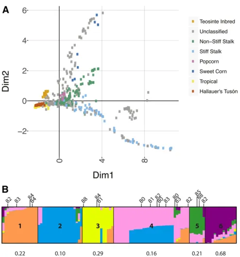
et al.2011) segregated within or among generations (Table 1). When compared to a global sample of maize, all of the individuals across generations of Hallauer’s Tusón clustered with tropical germplasm (Figure 2a), notwithstanding the temperate-adapted phenome of individuals belonging to the later generations (Teixeiraet al.2015). Thus, to tackle chal-lenges associated with crop vulnerability through plant breed-ing, Hallauer’s Tusón highlights the adaptive potential of maize landrace populations, and provides a unique source of germplasm likely to contain novel alleles for temperate maize breeding programs.
Retrospective analysis reveals admixture during selection on a structured founder population
breeding history of Hallauer’s Tusón. Although generations showed some SNP-based differentiationðmean F^ST9¼0:014Þ, as expected for progeny generated by random mating among selected individuals, overall inbreeding was minimal
ð^FIT9¼0:021Þ. However, on a per generation basis,^FISwas noticeably higher in g0, where 26% of the markers signifi -cantly deviated from Hardy–Weinberg equilibrium, with 78% of those deviations being due to an excess of homozy-gotes (Table 1). This suggested a Wahlund effect (Hartl and Clark 2007) from sampling geographically separated acces-sions that remained after the intermating step to formg0, but subsequent generations showed evidence of random mat-ing durmat-ing selection (Table 1).
STRUCTUREanalysis also indicated that individuals ing0 had formed largely by intermating within separate founder accessions and hybridization between specific pairs of acces-sions (Figure 2b and Table S3). Thesefindings are congruent with the way in which g0 was bred, whereby the original Tusón accessions were planted in adjoining blocks and allowed to open-pollinate, which would have favored mating within and between pairs of subpopulations. Although selec-tion could potentially favor specific subpopulations under these conditions, the genomic ancestral composition for g2 individuals showed admixture profiles that were propor-tional to that of the subpopulation sizes in g0 (Table S4). Thus, randomized bulking and planting of seed between each generation of artificial selection minimized subsequent in-breeding and population structure during selection.
Differentiation across a fraction of the genome potentiated strong phenotypic change
A decade of directional phenotypic selection, resulting in an overall mean decrease of 26 days to female-flowering time, caused generations to become strongly differentiated pheno-typically, as measured byQST(Figure 3). Simulation of neu-tral allele frequency changes that would occur under the breeding scheme used for phenotypic selection allowed us to identify 6115 of 43;628 ð14%Þmarkers with non-neutral allele frequency changes (referred to as SIMþ markers). These markers were widely dispersed across the genome (but with some clusters of linked SIMþmarkers, as described
later), and were distinguished from SIM2 markers by their increasing levels of^FHSTacross generations relative tog0 (Fig-ure 3). The identification of a sizeable fraction of genome-wide markers as SIMþsuggested afinite polygenic architec-ture (i.e., possibly tens to hundreds of loci affectingflowering time) could underlie the phenotypic response to selection. Similarly, based on QST2FST comparisons, the very large increases inQ^ST could be explained by much smaller levels ofF^STamplified across a large number of loci.
Population genetic analysis pinpoints shifts in the genetic architecture underlying response to selection
AlthoughF^ST increased overall across generations at SIMþ markers, changes in the frequencies of alleles at a locus var-ied mostly among generations. Using the simulator to test for non-neutral allele frequency changes between sequential pairs of generations showed that a majority of marker-specific departures were exclusive to one consecutive pair (Figure S3). This was coincident with the common observation of“bursts”in allele frequency change within a few generations, rather than monotonic changes across all generations (Figure S4, A–C).
Because transient changes in allele frequency were a prom-inent feature of the genomic response to selection, we used clustering to examine the temporal structure of allele frequen-cies among SIMþmarkers. A total of 15 allele frequency profile clusters (AFPCs) were resolved with a high degree of overall clustering structure (divisive coefficient = 0.98; Figure S5). Minor alleles ing0 with negative frequency trajectories were captured in AFPCs 123 comprising 10% of the SIMþ markers. The remaining g0 minor alleles, however, were enriched from starting frequencies that spanned the minor-allele frequency spectrum. Across clusters, some notable tran-sitions in allele frequency responses were observed: (i) alleles in AFPC1, which included the photoperiod sensitive allele (ZmCCT10-s), substantially reduced in frequency to become rare or removed within thefirst four generations; (ii) several AFPCs (6, 10, 11, 13, 14, and 15) showed clear increases in allele frequency within the first few generations that were limited thereafter; and (iii) for AFPC4, a dominant cluster comprising 43% of all SIMþmarkers, initially rare alleles ap-preciably increased afterg4.
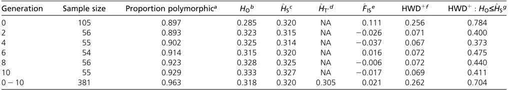
Table 1 Summary statistics for molecular genetic diversity in Hallauer’s Tusón
Generation Sample size Proportion polymorphica HOb H^Sc H^T9d ^FISe HWDþf HWDþ:HO£H^Sg
0 105 0.897 0.285 0.320 NA 0.111 0.256 0.784
2 56 0.893 0.323 0.315 NA 20.026 0.071 0.400
4 55 0.902 0.325 0.314 NA 20.037 0.067 0.373
6 54 0.914 0.315 0.320 NA 0.016 0.072 0.475
8 56 0.923 0.328 0.325 NA 20.006 0.072 0.440
10 55 0.929 0.333 0.327 NA 20.017 0.069 0.411
0210 381 0.963 0.318 0.320 0.305 0.021 0.262 0.704
aResults in the column are based on 49,477 markers (Table S1), while all remaining results are based on 44;445 markers with a minor variant count$12 among all samples. bAverage observed heterozygosity within generations. For all samples, this corresponds to the average among generations.
cAverage expected heterozygosity within generations. For all samples, this corresponds to the average among generations. dAverage expected heterozygosity for the total population.
eAverage inbreeding coefficient within generations. For all samples, this is^F
IT0, the average inbreeding coefficient for the total population. fThe proportion of markers that significantly deviated from Hardy–Weinberg equilibrium determined at a 5% FDR.
There were few instances, likeZmCCT10-s, where alleles were purged from the population. The loss of SNP variants in Hallauer’s Tusón was actually rare—1:0%ðn¼439 markersÞ of all SNPs ing0 were purged during selection (10 of these were SIMþ), and this was 3.4 times less than the average proportion of SNPs purged across replicate simulations of neutral frequency changeðrange:2:8%24:0%Þ. Taken to-gether, population genetic analysis suggested that selected genotype–phenotype relationships temporally shifted across a finite polygenic architecture with a predominant enrich-ment of initially minor alleles, resulting in the maintenance of genetic variation.
Quantitative genetic analysis contextualizes genome-wide population genetic dynamics
Our experimental design included phenotypic data on self-pollinated families of genotyped individuals sampled across generations evaluated in common environments (Figure 1), permitting estimation of quantitative genetic parameters and interpretation in the context of population genetic results. Underlying a 50-day range for female-flowering time in Hal-lauer’s Tusón, high broad and narrow sense heritabilities
ðH2¼0:9660:01:h2¼0:8160:08Þindicated a large fraction
of the phenotypic variance could be explained by genotypic effects, and the genotypic variance partitioned into 85% ad-ditive and 15% dominance variance with no residual genetic variance remaining. Including an additive-by-additive epi-static relationship matrix did not improve the modelfit nor did it explain any of the genotypic variance.
The genetic variance explained by individual chromosomes varied widely (Table S6). For instance, chromosome 10, in which theZmCCT10-associated causal variant is located, was an outlier that accounted for a large proportionð28%Þof the additive variance, while chromosome 2 included no additive or dominance variance. This supports and extends the pop-ulation genetic inference of a finite polygenic architecture, showing variability in the genetic effects across the genome available for selection.
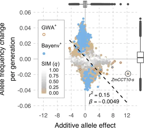
Genome-wide additive allele effects (estimated among families across generations) correlated with average changes in allele frequency per generationðr¼ 20:39;p,2:2e216Þ, whereby, as expected, alleles with negative effects on
female-flowering time (contributing to earlyflowering) tended to have positive slopes in allele frequency change and vice versa (Figure 4; the Bayenv and GWA hits highlighted in the Figure are dis-cussed in the next section). This relationship was largely driven by SIMþ markers, which accounted for 60% of the additive variance (none of the dominance variance)—an excessive en-richment given these constituted14% of the SNPs.
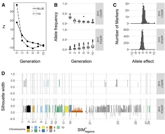
Nonlinear changes in the phenotypic mean and additive variance for female-flowering time across generations reflected some of the observed dynamics in allele frequency change (Figure 5). Changes in the mean could be modeled as a cubic function with significant ða¼0:05Þ coefficients
½fðxÞ ¼ 20:07gen3þ1:39gen229:64genþ100:27, where female-flowering time decreased across all generations but to a larger degree between generations 024 and 8210. These generations contained greater numbers of SIMþmarkers with larger magnitudes of allele frequency change (Figure S4d). The corresponding change in additive variance could be modeled as a quadratic function of generations with significant coefficients
½fðxÞ ¼ 214:11gen2þ1:06genþ31:58, where initially the variance was greatly reduced but later increased across gener-ations 6210; byg10, the additive variance exceeded that ofg4. These changes were coincident with initial reductions in the frequencies of few relatively large positive effect alleles (AFPC1) and subsequent enrichment of many rare negative effect alleles (AFPC4) (Figure 5 and Figure S5).
Robust selection and association mapping identify associations with keyflowering time genes
The simulation test clearly enriched for markers that differ-entiated generations (Figure 3), but not all of these are necessarily linked to causal variants underlying
female-flowering time selection. For instance, chromosome 2 cap-tured none of the genetic variance in female-flowering time; however, it contained SIMþmarkers (Table S6). The model used to simulate breeding events does not include compo-nents of potentially important sources of variation, such that Figure 2 Genetic diversity and population structure in Hallauer’s Tusón.
departures from the null distribution may also be due to factors such as individual differences in gametic fitness, or the secondary selection that was exerted for other traits (Hallauer and Carena 2016). On the other hand, covariance between causal and neutral allele frequency changes may generate false positives (Coop et al. 2010). Although we could not control for deviations due the former, selection and association mapping tests that control for genomic back-ground effects were used to identify markers exhibiting ro-bust changes in allele frequency across generations and robust associations with trait variation among generations, respectively.
Prior to applying these tests, we assessed the transgenera-tional structure of LD across the genome using subsets of low-ascertainment biased markers with a standardized min-imum allele count per generation (Table S2). Linkage dis-equilibrium was examined for each combination of SIM2and SIMþmarkers. Based on all pairwise estimates of LD, median
r2 showed little variation across generations, and did not exceed 0.04 within chromosomes and 0.01 between chromo-somes (data not shown). At increasingly higher percentiles of ther2distribution, LD between pairs of SIMþmarkers within chromosomes (but not between chromosomes) was elevated relative to other combinations of SIM2 and SIMþ markers (Figure S6). We found that the heightened LD between SIMþ markers was restricted to local linkage blocks, and tended to increase across generations (Figure S6)—a hallmark footprint of selection.
Given that the structure of LD gave rise to nonindepend-ent sets of linked SIM hits, kernel regression was used to delimit 29 SIMþregionsencompassing 1008ð16%Þof the SIMþ markers (Table S5). The Bayenv test, which controls for genome-wide covariance in sample allele frequencies, pro-duced Bayes factor values that were correlated with the SIM test ðSpearman0s jrj ¼0:62Þ. The top 1% of Bayenv hits were located on all chromosomes and were present in most SIMþregions, with regions on chromosome 9 being heavily populated with Bayenvþmarkers (Figure 6 and Fig-ure S7). Similarly, the FITR test, which is conditioned by variance in allele frequency change estimated from the
sample, primarily implicated SIMþregions on chromosome 9 as robust outliers.
GWA mapping performed on mean female-flowering time resulted in few genome-wide significant associations, not-withstanding the SNP-based polygenic model that explained essentially all of the genotypic variance. Between 2 and 12 GWA hits were detected across 1–10% FDR thresholds (Table S7). All but one of these showed the expected rela-tionship between the sign for the additive allele effect and slope in frequency change (we note this one marker was on chromosome 2, which explained none of the genetic vari-ance when the whole chromosome was modeled under a polygenic architecture). However, no GWA hits were de-tected on chromosome 9 nor within any of the SIMþregions. The top GWA hit was the presence–absence causal variant forZmCCT10-regulated photoperiodism, which was also de-tected as hits by the SIM and Bayenv tests but not the FITR test. Otherwise, the strength of signals (slopesvs.effects) for top hits by selection and association mapping tests tended to differ (Figure 4).
Taken together, robust tests to dissect the genetic basis of the response to selection implicated a number of genes pre-viously associated (causally or as a candidate gene) with variation in flowering time and photoperiodism in maize, several of which are highlighted in Figure 6.
Evidence for multiple local haplotypes underlying the phenotypic response to selection
The transition from selection on common to rare alleles occurred at some of the same regions of the genome. For instance, SIMþregionson different chromosomes included SIMþ markers in both AFPC1 and AFPC4, in which allele frequen-cies showed strong shifts during different periods of selection (Figure 5). Similarly, at theZmCCT10locus, robust associa-tions were detected for SNPs that responded to selection even after the elimination of ZmCCT10-s. Pairwise LD between significant markers at theZmCCT10locus indicated two sep-arate haplotypes were responsive to selection (Figure 7). These results reinforce the conclusion of a finite polygenic architecture underlying the response to selection, and extend
Figure 3 Q^ST2^F H
that to suggest selection on multiple local haplotypes was an important aspect of short-term evolution.
Discussion
Genetic analysis of adaptation in crop species provides a lens into evolution and generates relevant information for plant breeding. Althoughflowering time phenology has been widely studied in plants (Junget al.2017), we are aware of no study (in plants) that has dissected the transgenerational genomic basis of adaptive evolution (here, forflowering phenology) in a population translocated to a new environment. We help close this knowledge gap by investigating a tropical landrace of maize that was adapted to a temperate environment across a decade of artificial selection (Teixeiraet al.2015; Hallauer and Carena 2016). Using an efficient study design (Figure 1; Wisseret al.2011), we simultaneously elucidated population and quantitative genetic components underlying the 10 gen-erations of selection required for the population to reach a state of phenological adaptation similar to modern temperate maize lines.
The evolutionary capacity of the tropical Tusón landrace to become rapidly adapted to a temperate environment was attributed to afinite polygenic architecture, yet two genomic phases underlying the phenotypic response to selection could be discerned. Thefirst phase, from generations 024;was
distinguished by an oligogenic-like architecture, where marked reductions of a relatively small number of moder-ate-frequency minor variants in g0 (AFPCs 1 and 2), with relatively large positive effects onflowering time, contributed to an initial strong response to phenotypic selection and a large reduction in genetic variance (Figure 5). Afterward, the genomic basis of the response transitioned to become dominated by the enrichment of a large number of rare-minor variants in g0 with smaller-sized negative effects on
flowering time, leading to a genome-wide increase in hetero-zygosity (Table 1) and consequent increase in additive vari-ance (Figure 5).
The observed changes in phenotypic mean and variance are similar to expected outcomes theorized for a finite polygenic architecture with additive allele effects (Chevalet 1994). Consistent with an additive genetic model, several AFPCs showed linear trends across all generations reflective of un-conditionally (un)favorable alleles in Hallauer’s Tusón (Fig-ure S5). However, AFPCs with transient shifts in allele frequency were also detected, such as mid-to-late genera-tional responses and plateaus in allele frequency change, highlighting a context-dependent component of the genetic architecture underlying the response to phenotypic selection. The same pattern of plateauing allele frequencies after an initially strong shift was found by temporal analysis of natu-ral populations of Drosophila melanogaster adapted to a novel laboratory environment, which Orozco-terWengelet al.
(2012) reasoned was due to overdominant or antagonistic pleiotropic effects. It has been demonstrated (mathemati-cally) that the selection coefficient for an additive allele can vary across generations also as a result of changes in back-ground polygenic variance (Chevin and Hospital 2008). The genotypic variance in Hallauer’s Tusón partitioned into addi-tive (primarily) and dominance genetic variance with no ap-parent epistatic genetic variance, but epistatic genetic effects will contribute to the additive genetic variance component in many cases, such that inferences about gene action should not be drawn from variance components estimates (Hillet al.
2008; Huang and Mackay 2016). Thus far, genetic studies on
flowering time in maize have described an architecture with predominantly additive genetic variance (e.g., Buckleret al.
2009; Coleset al.2010; note that these studies use inbred lines, which precludes estimation of dominance variance), but reports of dominant, overdominant (Coles et al.2011) and epsistatic (Blancet al.2006; Durandet al.2012) allele effects on variation in flowering characteristics also exist. With a limited sample size for quantitative genetic dissection per generation, our study is unable to clarify the causes or relative contribution of context-dependent effects on the re-sponse to phenotypic selection.
Maize is highly diverse (Buckleret al.2006), and landraces of maize are locally adapted to a wide range of environments (Committee on The Preservation of Indigenous Strains of Maize 1952–1963). Still, it was surprising that Hallauer’s Tusón captured nearly all of the SNPs on the MaizeSNP50 chip (Ganalet al.2011). This high level of molecular genetic Figure 4 Genome-wide relationship between slopes in allele frequency
variation, as well as the detection of an increasing proportion of polymorphic platform SNPs across generations (Table 1), led us to question whether migrant pollen had entered the population, particularly since it was open-pollinated during selection; although the population was bred in spatial and temporal isolation of other maize populations. Separate lines of evidence indicate the population could have very high di-versity while remaining a closed system with no migration or pollen flow. First, similar to ourfinding, another study has found that individual populations of maize landraces can capture .90% of the SNPs on the same MaizeSNP50 plat-form (Arteagaet al.2016). Because the base population of Hallauer’s Tusón was admixed from multiple, geographically dispersed populations of the landrace Tusón, there is a greater likelihood for the level of diversity to be high. Second, the binomial sampling probabilities for our study limited detection of rare variants within generations despite their putative presence in the population. For instance, based on our sample sizes (which was larger for g0), SNPs at a frequency of 1% have an 11% chance of being undetected in g0 and a 33% chance of being undetected in the other generations, but subtle increases above 1% result in large increases in the probability of their detection. Therefore, variants that were not detected in one generation but de-tected in another may exist at low frequencies, and the transgenerational increase in polymorphic platform SNPs can be explained by selection of initially rare alleles. Finally, considering the most frequent migrant sources in Iowa where the population was selected would be of temperate origin, all of the genotyped individuals in Hallauer’s Tusón
clustered with other maize samples of tropical rather than temperate origin (Figure 2).
A fundamental question in genetics is how populations acquire and maintain variation that conditions them with the capacity to adapt to a novel environment. At the locations where the source populations were already adapted and grown, we presume stabilizing selection occurred onfl ower-ing time, asflowering time affectsfitness in an environmen-tally dependent manner (Hall and Willis 2006; Mercer and Perales 2019). Stabilizing selection is expected to deplete genetic variation (Barton and Keightley 2002), such that the extensive functional variation for flowering time in Hallauer’s Tusón suggests evolutionary forces beyond mutation and selection for a single optimalflowering time affected the founding populations. Teixeira et al. (2015) showed that
flowering time variation in Hallauer’s Tusón is under strong genetic and environmental control, with relatively little ge-notype-by-environment interaction (however, GxE effects were present across latitude and greater in the initial gener-ations). Therefore, seasonalfluctuations that affect the rela-tionship betweenflowering time andfitness (Giauffretet al.
2000) and multivariate constraints to evolution (Walsh and Blows 2009) likely contributed to the maintenance of sub-stantial standing variation for this trait, and therefore its ca-pacity for adaptation to a novel environment.
As the population was subjected to directional selection in a temperate environment, alleles contributing to earlier
frequent variants such as the photoperiod insensitive allele
ZmCCT10-i (present at 75% ing0), most of theseð75%Þ existed in the minor frequency domain. This was in con-trast to minor alleles in g0 at SIM2 markers, for which
50% had negative effects on flowering time. Hence, in the base generation of Hallauer’s Tusón, favorable alleles for temperate adaptation primarily exist in the minor fre-quency spectrum.
Due to the admixture of multiple Tusón populations to formg0, however, the allele frequencies reflect those among (not within) the founder populations, such that native pop-ulation allele frequencies of temperate-adaptive variants are confounded. To address this, subpopulation assignments for samples from g0 (assumed to correspond to the founding populations) were used to compute subpopulation-specific allele frequencies for the corresponding minor allele in the wholeg0sample (data not shown). Across all SIMþmarkers, most alleles were shared among multiple subpopulations; only 8% of these markers included private alleles. This suggests that geographically separated populations of the landrace Tusón have retained shared alleles that enable lat-itudinal adaptation, afinding that is congruent with geographical
association results from a diverse sample of maize landraces (Romero Navarroet al.2017).
Our inference from allele frequency data, however, should be considered with caution. The inferred number of loci (finite polygenic architecture) and effect of selection on variants across the allele frequency spectrum is based on markers that are unlikely to be causal variants themselves, but are expected to tag local haplotype blocks containing causal variants (Nuzhdin and Turner 2013; Kelly and Hughes 2019). More-over, any initially rare variants with late flowering time effects would likely have been purged or kept at low frequencies, leading to low power of detection for both selec-tion and associaselec-tion mapping, despite the importance of such potential variants for environmental adaptation. This repre-sents a bias to evolutionary inference in experimentally evolved populations and highlights the need for deeper sam-pling within generations and other approaches to elucidate the structure of natural variation for adaptation.
Our study design allows for the mapping and character-ization of specific genomic loci underlying phenotypic evolu-tion. Although the relatively small sample ð300 familiesÞ and low marker density (tens of thousands of SNPs) limited Figure 7 Allele frequency change and linkage disequilibrium at ZmCCT10. (A) Variant frequency change (y-axis) across generations (x -axis) for the nearestfive markersflanking the ZmCCT10_CACTA causal site. Points are color coded according to the combination of test results (ZmCCT10_CACTA was positive for the SIM, Bayenv and GWA tests and is color coded red). (B) Pairwise LD between the markers in (A). Marker distances from the insertion site for ZmCCT10_CACTA (AGPv4 94,435,768) are indicated. Negative values are in the direction of theZmCCT10 transcrip-tion start site.
the power of our study, we nevertheless detected robust as-sociations with known genes involved inflowering time ad-aptation, raising confidence in our discovery of other unique loci (Figure S7). For instance, selection against photoperiod sensitivity was a major component of adaptation in Hallauer’s Tusón (Teixeira et al.2015). Regions encompassing ZCN8,
CONZ1,COL9,CRY2, andZmCCT9on chromosomes 8 and 9, and a causal regulatory variant ofZmCCT10on chromosome 10, were detected by selection or association mapping (Fig-ure 6). These genes are regulators of photoperiodism in plants (Guo et al. 1989; Cheng and Wang 2005; Miller
et al.2008; Menget al.2011) that have contributed to lat-itudinal adaptation (Yanget al.2013; Guoet al.2018; Huang
et al. 2018), all of which were identified in a large-scale mapping study on photoperiod sensitivity in maize (cf. Figure 6 and Figure 2 in Hunget al.2012). Moreover, we found that different local haplotypes were responsive to selection at sev-eral of these same loci where Hung et al.(2012) detected allelic series [e.g., SIMþregions21223 and 25 (Figure 5) and theZmCCT10locus (Figure 7)]. On chromosome 8, no robust association was detected for the Vegetative to Generative Transition 1(VGT1) gene (Salviet al.2007) involved in ear-liness per se, but a maize homolog ofArabidopsis thaliana de-etiolated 1 (DET1) involved in photomorphogenesis (Pepper et al. 1994), not previously highlighted for maize adaptation, mapped to a conspicuous SIMþregion across the centromere of the chromosome.
Development of next-generation crop varieties is crucial to ensuring ample production and quality of plant-based prod-ucts for society. Reliance on limited pools of diversity for breeding and the creation of monocultures can lead to con-strained and vulnerable production systems, but genetic di-versity is ecologically structured whereby alleles that could be useful in a target production environment reside in germ-plasm that suffers from maladaptive syndromes (Teixeira
et al.2015). Our study shows the potential for maize land-races to be adapted to temperate environments by simple recurrent selection for earlyflowering time while resulting in minimal loss of molecular genetic variation to reach the adapted state. The lack of a linked footprint of selection
ðSIMþregionÞ encompassing the ZmCCT10 causal site, which had the strongest association withflowering time and under-went a rapid complete-sweep, suggests that some critical adaptive mutations in maize are embedded in regions of low LD, which would permit the maintenance of linked var-iation during directional selection. Moreover, the multidi-mensional nature of the genetic architecture underlying response tophenotypicselection, involving multiple loci and alleles with context-dependent effects, appears to enable a rapid shift toward an adapted state with limited loss in di-versity. We anticipate that further characterization of these additional layers of the genetic architecture and dynamics of the genomic response to selection will lead to new advances in genomic prediction across generations. By bridging popu-lation and quantitative genetic inference, this study advances our understanding of short-term evolution, providing unique
insights that aid in developing approaches to adapt crops to climate change.
Acknowledgments
We thank Michael Dumas (University of Delaware) who produced genotype data for theZmCCT10causal site. R.J.W. thanks Keith Hopper (USDA-ARS) for meetings at Iron Hill where this work was discussed at length. This project was supported by Agriculture and Food Research Initiative Grant No. 2011-67003-30342 from the United States Department of Agriculture (USDA) National Institute of Food and Agri-culture (AgriAgri-culture and Natural Resources Science for Cli-mate Variability and Change Program).
Author contributions: A.H. created the original recurrently selected population. R.J.W., J.B.H., N.d.L., S.F.-G., N.L., S.C.M., and W.X. designed the study and conducted field experiments, while T.W. assisted with coordination. J.E.C.T. led the genotyping project and contributed intellectually. R.J.W. and J.D. developed the whole genome simulator. R.J.W., Z.F., and J.B.H. developed analysis procedures and analyzed the data. R.J.W. and J.B.H. interpreted the results and wrote the paper, with contributions from Z.F. All authors except T.W. and A.H. edited the manuscript.
Literature Cited
Arteaga, M. C., A. Moreno-Letelier, A. Mastretta-Yanes, A. Vázquez-Lobo, A. Breña-Ochoa et al., 2016 Genomic variation in re-cently collected maize landraces from Mexico. Genom. Data 7: 38–45.https://doi.org/10.1016/j.gdata.2015.11.002
Barrick, J. E., and R. E. Lenski, 2013 Genome dynamics during experimental evolution. Nat. Rev. Genet. 14: 827–839.https:// doi.org/10.1038/nrg3564
Barton, N. H., and P. D. Keightley, 2002 Understanding quantita-tive genetic variation. Nat. Rev. Genet. 3: 11–21. https:// doi.org/10.1038/nrg700
Barton, N. H., A. M. Etheridge, and A. Véber, 2017 The infi nites-imal model: definition, derivation, and implications. Theor. Popul. Biol. 118: 50–73.https://doi.org/10.1016/j.tpb.2017.06.001
Baxter, S. W., F. R. Badenes-Pérez, A. Morrison, H. Vogel, N. Crick-more et al., 2011 Parallel evolution of Bacillus thuringiensis
toxin resistance in Lepidoptera. Genetics 189: 675–679.
https://doi.org/10.1534/genetics.111.130971
Benjamini, Y., and Y. Hochberg, 1995 Controlling the false dis-covery rate: a practical and powerful approach to multiple test-ing. J. R. Stat. Soc. B 57: 289–300.
Berg, J. J., and G. Coop, 2014 A population genetic signal of poly-genic adaptation. PLoS Genet. 10: e1004412.https://doi.org/ 10.1371/journal.pgen.1004412
Bhatia, G., N. Patterson, S. Sankararaman, and A. Price, 2013 Estimating and interpreting FST: the impact of rare variants. Genome Res. 23: 1514–1521.https://doi.org/10.1101/gr.154831.113
Blanc, G., A. Charcosset, B. Mangin, A. Gallais, and L. Moreau, 2006 Connected populations for detecting quantitative trait loci and testing for epistasis: an application in maize. Theor. Appl. Genet. 113: 206–224. https://doi.org/10.1007/s00122-006-0287-1
Bradbury, P. J., Z. Zhang, D. E. Kroon, T. M. Casstevens, Y. Ramdoss
complex traits in diverse samples. Bioinformatics 23: 2633– 2635.https://doi.org/10.1093/bioinformatics/btm308
Buckler, E. S., B. S. Gaut, and M. D. McMullen, 2006 Molecular and functional diversity of maize. Curr. Opin. Plant Biol. 9: 172– 176.https://doi.org/10.1016/j.pbi.2006.01.013
Buckler, E. S., J. B. Holland, P. J. Bradbury, C. B. Acharya, P. J. Brownet al., 2009 The genetic architecture of maizeflowering time. Science 325: 714–718.https://doi.org/10.1126/science. 1174276
Bulmer, M. G., 1971 The effect of selection on genetic variability. Am. Nat. 105: 201–211.https://doi.org/10.1086/282718
Burke, M. K., and A. D. Long, 2012 What paths do advantageous alleles take during short-term evolutionary change? Mol. Ecol. 21: 4913–4916.https://doi.org/10.1111/j.1365-294X.2012.05745.x
Burke, M. K., J. P. Dunham, P. Shahrestani, K. R. Thornton, M. R. Roseet al., 2010 Genome-wide analysis of a long-term evolu-tion experiment withDrosophila. Nature 467: 587–590.https:// doi.org/10.1038/nature09352
Chan, Y. F., F. C. Jones, E. McConnell, J. Bryk, L. Büngeret al., 2012 Parallel selection mapping using artificially selected mice reveals body weight control loci. Curr. Biol. 22: 794–800.
https://doi.org/10.1016/j.cub.2012.03.011
Chardon, F., L. Moreau, M. Falque, J. Joets, L. Decousset et al., 2004 Genetic architecture of flowering time in maize as in-ferred from quantitative trait loci meta-analysis and synteny conservation with the rice genome. Genetics 168: 2169–2185.
https://doi.org/10.1534/genetics.104.032375
Cheng, X. F., and Z. Y. Wang, 2005 Overexpression ofCOL9, a
CONSTANS-LIKEgene, delaysflowering by reducing expression of CO andFT in Arabidopsis thaliana. Plant J. 43: 758–768.
https://doi.org/10.1111/j.1365-313X.2005.02491.x
Chevalet, C., 1994 An approximate theory of selection assuming a
finite number of quantitative trait loci. Genet. Sel. Evol. 26: 379–400.https://doi.org/10.1186/1297-9686-26-5-379
Chevin, L. M., and F. Hospital, 2008 Selective sweep at a quanti-tative trait locus in the presence of background genetic varia-tion. Genetics 180: 1645–1660. https://doi.org/10.1534/ genetics.108.093351
Coles, N. D., M. D. McMullen, P. J. Balint-Kurti, R. C. Pratt, and J. B. Holland, 2010 Genetic control of photoperiod sensitivity in maize revealed by joint multiple population analysis. Genetics 184: 799–812.https://doi.org/10.1534/genetics.109.110304
Coles, N. D., C. T. Zila, and J. B. Holland, 2011 Allelic effect variation at key photoperiod response quantitative trait loci in maize. Crop Sci. 51: 1036–1049. https://doi.org/10.2135/ cropsci2010.08.0488
Committee on The Preservation of Indigenous Strains of Maize monographs on Races of Maize (1952–1963). National Acad-emy of Sciences—National Research, Washington, D.C. Pub. N 1136 (Venezuela); Pub. N 510 (Columbia); Pub. N 511 (Central America); Pub. N 593 (Brazil and other Eastern South American Countries); Pub. N 747 (Bolivia); Pub. N 792 (West Indies); Pub. N 847 (Chile); Pub. N 915 (Peru); Pub. N 975 (Ecuador); Pub. N 453 (Cuba); and Races of Maize in Mexico by the Bussey Institute, Harvard University, MA.
Coop, G., D. Witonsky, A. Di Rienzo, and J. K. Pritchard, 2010 Using environmental correlations to identify loci under-lying local adaptation. Genetics 185: 1411–1423. https:// doi.org/10.1534/genetics.110.114819
Darwin, C., 1859 On the Origin of Species by Means of Natural Selection, or,the Preservation of Favoured Races in the Struggle for Life. John Murray, London.
Ducrocq, S., D. Madur, J. Veyrieras, L. Camus-Kulandaivelu, M. Kloiber-Maitz et al., 2008 Key impact of Vgt1 on flowering time adaptation in maize: evidence from association mapping and ecogeographical information. Genetics 178: 2433–2437.
https://doi.org/10.1534/genetics.107.084830
Durand, E., S. Bouchet, P. Bertin, A. Ressayre, P. Jamin et al., 2012 Flowering time in maize: linkage and epistasis at a major effect locus. Genetics 190: 1547–1562.https://doi.org/10.1534/ genetics.111.136903
Durand, E., M. I. Tenaillon, X. Raffoux, S. Thépot, M. Falqueet al., 2015 Dearth of polymorphism associated with a sustained re-sponse to selection forflowering time in maize. BMC Evol. Biol. 15: 103.https://doi.org/10.1186/s12862-015-0382-5
Evanno, G., S. Regnaut, and J. Goudet, 2005 Detecting the num-ber of clusters of individuals using the software STRUCTURE: a simulation study. Mol. Ecol. 14: 2611–2620. https://doi.org/ 10.1111/j.1365-294X.2005.02553.x
Falconer, D. S., and T. F. C. Mackay, 1996 Introduction to Quan-titative Genetics, Ed. 4. Pearson, Essex.
Fernando, R. L., C. Stricker, and R. C. Elston, 1994 The finite polygenic mixed model: an alternative formulation for the mixed model of inheritance. Theor. Appl. Genet. 88: 573–580.
https://doi.org/10.1007/BF01240920
Fisher, R. A., 1918 The correlation between relatives on the sup-position of Mendelian inheritance. Trans. R. Soc. Edinb. 52: 399–433.https://doi.org/10.1017/S0080456800012163
Frascaroli, E., T. A. Schrag, and A. E. Melchinger, 2013 Genetic diversity analysis of elite European maize (Zea mays L.) inbred lines using AFLP, SSR, and SNP markers reveals ascertainment bias for a subset of SNPs. Theor. Appl. Genet. 126: 133–141.
https://doi.org/10.1007/s00122-012-1968-6
Ganal, M. W., G. Durstewitz, A. Polley, A. Bérard, E. S. Buckler
et al., 2011 A large maize (Zea mays L.) SNP genotyping ar-ray: development and germplasm genotyping, and genetic map-ping to compare with the B73 reference genome. PLoS One 6: e28334.https://doi.org/10.1371/journal.pone.0028334
Giauffret, C., J. Lothrop, D. Dorvillez, B. Gouesnard, and M. De-rieux, 2000 Genotype x environment interactions in maize hy-brids from temperate or highland tropical origin. Crop Sci. 40: 1004–1012.https://doi.org/10.2135/cropsci2000.4041004x
Gilmour, A. R., B. J. Gogel, B. R. Cullis, and R. Thompson, 2009 ASReml user guide release 3.0. Hemel Hemptead: VSN International Ltd.
Goodman, M., 1998 Research policies thwart potential payoff of exotic germplasm. Diversity (Basel) 14: 30–35.
Goodman, M. M., and W. L. Brown, 1988 Races of corn, pp. 33– 74 inCorn and Corn Improvement, Ed. 3, Chap. 2, edited by G. F. Sprague and J. W. Dudley. American Society of Agronomy, Crop Science Society of America, Soil Science Society of America, Madison, WI.
Goudet, J., 2005 HIERFSTAT, a package for R to compute and test hierarchical F-statistics. Mol. Ecol. Notes 5: 184–186.https:// doi.org/10.1111/j.1471-8286.2004.00828.x
Graffelman, J., 2015 Exploring diallelic genetic markers: the HardyWeinberg package. J. Stat. Softw. 64: 1–23.https://doi.org/ 10.18637/jss.v064.i03
Guo, H., H. Yang, T. C. Mockler, and C. Lin, 1989 Regulation of
flowering time by Arabidopsis photoreceptors. Science 279: 1360–1363.https://doi.org/10.1126/science.279.5355.1360
Guo, L., X. Wang, M. Zhao, C. Huang, C. Liet al., 2018 Stepwise cis-regulatory changes in ZCN8 contribute to maizefl owering-time adaptation. Curr. Biol. 28: 3005–3015.e4.https://doi.org/ 10.1016/j.cub.2018.07.029
Hall, M. C., and J. H. Willis, 2006 Divergent selection onfl ower-ing time contributes to local adaptation in Mimulus guttatus
populations. Evolution 60: 2466–2477.https://doi.org/10.1111/ j.0014-3820.2006.tb01882.x
Hallauer, A. R., and M. J. Carena, 2016 Registration of BS39 maize germplasm. J. Plant Regist. 10: 296–300.https://doi.org/10.3198/ jpr2015.02.0008crg