Implicit Traffic Classification for Service Differentiation
Chintan Trivedi H. Joel Trussell Arne Nilsson Mo-Yuen Chow
Department of Electrical and Computer Engineering NC State University
Raleigh, NC 27695-7911
Email: {crtrived, hjt, nilsson, chow}@eos.ncsu.edu
Corresponding Author: Arne Nilsson (Phone- +1 919 515 5130, Fax- +1 919 515 5523)
Abstract – Current trends indicate that traffic handling in the networks of the next generation
will include service differentiation. Traffic classification is a fundamental problem to be solved before this objective can be achieved. In this work we propose a unique scheme to classify Internet traffic into flows over a time frame, based on the application to which the packets belong. One key aspect of our scheme is that it does not involve reading the OSI layer 4 header to determine the application. This ‘implicit’ classification builds a foundation for estimation and prediction of traffic mix, which is a long-term goal of this research project. The classification results mentioned in this paper indicate that this approach is promising.
I. INTRODUCTION AND MOTIVATION
Over the last few years, traffic on the Internet has proliferated, both in terms of amount of traffic, and in variety of applications. The introduction of voice, video and other real-time applications has changed the way the Internet is used. This has triggered the need for a change in traffic handling on the Internet. In particular, there is increasing demand for service differentiation. The Diffserv architecture[8] of the IETF is one such step towards fulfilling this demand. However, for any such service, the very basic problem one encounters is that of classification. The traffic on the Internet can be classified using various parameters, viz. source and/or destination IP address (or prefix), type-of-service, application, etc. A number of classification schemes are discussed in [1][5][6][7]. In this work, we classify the Internet traffic based on the application to which the packets belong. An easy approach to do so is by extracting the port number information from the layer 4 (TCP/UDP) header [4]. However, there are certain problems with this approach. With the introduction of the Network Address Port Translation (NAPT) concept, the port numbers are no longer a trustworthy source for determining the application type. In a free environment like the Internet, it is not mandatory for applications to use specific port numbers[2]. It is very likely that other applications would spoof port numbers in order to gain better service. Also, future network security algorithms might encrypt even the packet headers, along with the data contained in the packet. These bottlenecks motivate our approach in classifying and modeling network traffic. In this paper, we classify IP traffic into different application types on the basis of packet attributes obtainable at OSI layer 3 (i.e. IP layer). These attributes are intrinsic characteristics of the packet itself. Also, it should be noted that we do not classify the traffic on a per-packet basis, rather the traffic flows are classified.
The paper is organized as follows. Section II describes the data used in our analysis. Section III describes in detail our approach to classification, the experiments we conducted, and the results we obtained. Section IV concludes the analysis with a discussion of future work.
II. DATA USED IN ANALYSIS
Our requirement was to use packet attributes that cannot be spoofed by the source. The ones that we considered using were the source and destination IP address pairs, packet size and inter-arrival time. But as our goal was to classify the traffic based on the application, the IP address-pair option was dropped and we decided on using packet size and inter-arrival time.
The second question was that of the level at which to classify. Performing classification on a per-packet basis was not possible because the attributes we selected do not allow us to do so. To be more precise, packets from different applications can have the same packet sizes and inter-arrival times. So we decided to classify the flows, i.e. classify the traffic over a time frame.
The data for this project is collected from the North Carolina State University backbone network using TCPDUMP software. The data is stored in the form of tab delimited text files. Each line in the file, similar to the fictitious line shown below, represents one data packet.
928215372.32805002 60 152.7.4.222 4248 206.162.67.254 80
The fields in sequence from left to right are: • Timestamp (in seconds)
• Packet size (in bytes) • Source IP Address • Source port number • Destination IP Address • Destination port number
The overall details of the data are as below:
• Each file has TCPDUMP trace of approximately 500,000 packets in it, and represents varying time durations - the minimum being 118 s, maximum 999 s. The average over all files is 372 s.
• The data is divided into two sets: Training set, and Test set (the reason for doing this will be clear later on)
• Each of these 2 sets has 8 sub-sets.
• Each of the 16(8x2) sub-sets contain 3 files, similar to the ones described above. The 3 files are obtained with an average time gap of 15 minutes between each of them.
• Each of the 8 data sets is selected with average time intervals of 968 minutes between them (approximately 16 hrs).
The first step towards classification is to determine the classes into which we will categorize. For our approach, these classes are the applications. We calculated the contribution of each application in the overall traffic mix across the entire training set, the result of which is given in Table 1. Here, a packet is considered to be belonging to an application if the source and/or destination port number in the packet header is of that application.
III. CLASSIFICATION
As mentioned before, our approach is to classify over a period of time. We studied the distribution of the features we selected, i.e. packet size and inter-arrival time, over periods of time spanning one sub-set.
TABLE 1
CONTRIBUTION OF DIFFERENT APPLICATIONS TO THE INTERNET TRAFFIC
Application Port Number Number of Packets % contribution
DNS 53 179960 1.50
FTP(data) 20 933777 7.78
HTTP 80 4290363 35.75
NNTP 119 560403 4.67
RESERVED 0 397384 3.31
SMTP 25 540878 4.51
TELNET 23 416830 3.47
All Other - 4681205 39.01
A. Packet size distribution
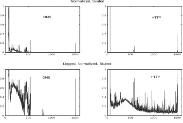
A histogram is computed to estimate the distribution of packet sizes for each application. For the initial analysis, a bin width of one was used. The sample plots are given in Fig. 1. It was observed that for most applications, the number of packets in the small packet-size range, i.e. between 60-80 bytes, was large. In fact, it is so large that if a graph used linear scaling on Y-axis, the lines for other packet sizes become almost invisible. Thus, logarithmic scaling is used to display the histograms.
0 500 1000 1500
0 0.2 0.4 0.6 0.8 1
0 500 1000 1500
0 0.2 0.4 0.6 0.8 1
0 500 1000 1500
0 0.2 0.4 0.6 0.8 1
0 500 1000 1500
0 0.2 0.4 0.6 0.8 1
DNS
DNS
HTTP
HTTP Normalized, Scaled
Logged, Normalized, Scaled
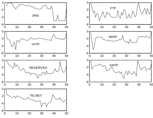
Based on the observation of fine resolution histograms, new bins were chosen for ease of computation. The entire range of packet sizes is divided into 50 bins and hence the packet-size distributions are vectors of dimension 50. The sizes of bins are not equal across the entire range of packet-sizes. They are narrow in the small packet-size region, where the packet-size distribution is dense, and increase toward the large packet-size region. The bin details are given below:
Bin No. Packet
size-bytes 1 0-65 2 66-70 3 71-75 4 76-80 5 81-85 6 86-90 7 91-95 8 96-100 9 101-105 10 106-120 11 121-135 12 136-150 13 151-165 14 166-180 15 181-195 16 196-210 17 211-225 18 226-240 19 241-255 20 256-270 21 271-285 22 286-300 23 301-315 24 316-330 25 331-345 26 346-360 27 361-375 28 376-390 29 391-405 30 406-420 31 421-435 32 436-450 33 451-465 34 466-480 35 481-495 36 496-510 37 511-525 38 526-540 39 541-570 40 571-600 41 601-700 42 701-800 43 801-900 44 901-1000 45 1001-1100 46 1101-1200 47 1201-1300 48 1301-1400 49 1401-1500 50 1501-1600
The plots of average packet size distribution across the entire training set are shown in Fig. 2. As explained before, the histogram is normalized and logged before plotting in order to magnify the large packet-size region.
0 10 20 30 40 50
-6 -4 -2 0
DNS
0 10 20 30 40 50
-6 -4 -2 0
FTP
0 10 20 30 40 50
-6 -4 -2 0
HTTP
0 10 20 30 40 50
-6 -4 -2 0
NNTP
0 10 20 30 40 50
-6 -4 -2 0
RESERVED
0 10 20 30 40 50
-6 -4 -2 0
SMTP
0 10 20 30 40 50
-6 -4 -2 0
TELNET
B. Inter-arrival time distribution
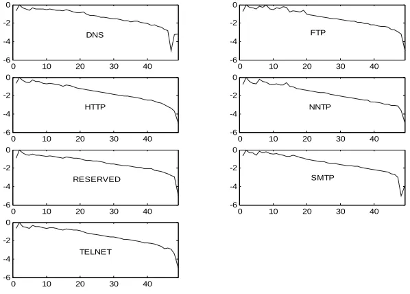
We used the same approach as in packet-size distributions to compute the histograms for inter-arrival time distributions, the only difference being that here we have 49 bins as compared to 50 in the packet-size case. The plots of average inter-arrival time distribution across the entire training set are shown in Fig. 3. As before, the histogram is normalized and logged before plotting in order to magnify the large inter-arrival time region.
0 10 20 30 40
-6 -4 -2 0
DNS
0 10 20 30 40
-6 -4 -2 0
FTP
0 10 20 30 40
-6 -4 -2 0
HTTP
0 10 20 30 40
-6 -4 -2 0
NNTP
0 10 20 30 40
-6 -4 -2 0
RESERVED
0 10 20 30 40
-6 -4 -2 0
SMTP
0 10 20 30 40
-6 -4 -2 0
TELNET
Fig. 3: Plots of histograms (normalized and logged) for inter-arrival time distributions (in 49 bins) of different applications.
C. Using both packet size and inter-arrival time information
The more information we add, the better the resulting classification should be. Following this principle, we thought of combining the packet size and inter-arrival time information. However, the results would be better only if the two variables are relatively uncorrelated. To investigate this, we calculated the correlation coefficient of packet size and inter-arrival time over the entire training set. Table 2 gives the average correlation coefficients between packet size and inter-arrival time for all applications across the training set. It is observed that the packet size and inter-arrival time are reasonably uncorrelated. Hence, we experimented with using a combination of the two as a variable.
TABLE 2
CORRELATION COEFFICIENTS BETWEEN PACKET SIZE AND INTER-ARRIVAL TIMES FOR DIFFERENT APPLICATIONS.
Application Correlation Coefficient
DNS 0.0368
FTP 0.1157
HTTP -0.0006
NNTP 0.1361
RESERVED -0.0374
SMTP 0.0928
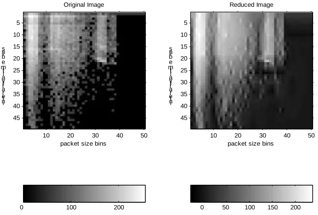
We did this using two approaches. In one, we generated a 2-D histogram matrix of dimension 49x50 for each application, where the rows indicated the packet size distributions, and columns the corresponding inter-arrival time distributions. Then we treated the matrix as an image, and used the Wavelet Toolbox of MATLAB to decompose the image into its wavelet coefficients. We eliminated the wavelet coefficients having the least standard deviation across the 56 vectors to compress the image, and then reconstructed it with the remaining coefficients. In this way, we could reduce the dimension of the variable vector from 2450 (49x50), to 250. In Fig. 4 we show an example of comparison of the two images. The first plot is the original figure, and the second is the one reconstructed using 250 wavelet coefficients.
In the second approach, we simply concatenate the packet-size distribution and inter-arrival time distribution vectors to form a single vector of dimension 99.
0 100 200
Original Image
packet size bins in
te r-arr iv al ti me bin s
10 20 30 40 50
5 10 15 20 25 30 35 40 45
0 50 100 150 200 Reduced Image
packet size bins in
te r-arr iv al ti me bin s
10 20 30 40 50
5 10 15 20 25 30 35 40 45
Fig. 4: Plots of images (original and compressed) for packet size vs. inter-arrival time distributions (in 50x49 matrices) of DNS
D. Clustering:
We used different clustering methods for this purpose. As clustering parameters, we used the packet size distribution, inter-arrival time distribution, and the combination of both (as described in detail in the previous section) as features. These distributions for all the 8 applications across the 8 data sets of the training set were used as instances of these features. Hence, for each feature, we have 64 data-points to cluster.
Note: In this analysis, we have used histograms that are logged and normalized as in the previous section. If 3 or more vectors of an application are clustered together and constitute a majority in the cluster, it is considered to be a valid cluster of that application. All others are considered as misclassifications.
The clustering results of the 64 packet-size distribution vectors using the Ward’s method are given in Table 3. The clustering based on inter-arrival time alone, and that using a combination of packet-size and inter-arrival time were poor. This might be expected from the similarities of the inter-arrival time histograms in Fig. 3.
TABLE 3
RESULTS OF CLUSTERING THE PACKET SIZE DISTRIBUTIONS
Cluster Number Members(Number/Application)
1 8 / HTTP
2 8 / DNS
3 8 / NNTP
4 8 / TELNET
5 8 / SMTP
6 8 / FTP
7 8 / RESERVED
8 8/ All Other
Since the packet size distributions gave better clustering results, while at the same time using less information as compared to the 2-D case, we decided to go ahead with the packet size distributions as our classification parameter.
E. Reducing the size of data set for training:
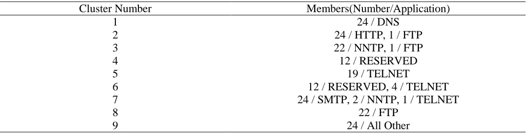
Next, we tried to optimize the performance of the classification scheme by using smaller data sets, and thus obtain a trade-off between data set size and classification efficiency. Instead of using 3 files in a sub-set, we performed a similar analysis using 1 file, i.e. the size of the data used was reduced to 1/3rdas that of the original. The clustering results with this reduced data are given in Table 4.
It is noted that in Table 4, the RESERVED data falls into two separate clusters. This is acceptable since there is no mixing in the clusters. It does indicate that this class is not homogenous. Here, we see that according to our criterion of successful clustering, we have 9 misclassifications out of a total of 192(8x24) vectors used. However, considering the fact that we have used only one-third of the data, the result is quite satisfactory.
TABLE 4
RESULTS OF CLUSTERING THE PACKET SIZE DISTRIBUTIONS USING REDUCED DATA SETS
Cluster Number Members(Number/Application)
1 24 / DNS
2 24 / HTTP, 1 / FTP
3 22 / NNTP, 1 / FTP
4 12 / RESERVED
5 19 / TELNET
6 12 / RESERVED, 4 / TELNET
7 24 / SMTP, 2 / NNTP, 1 / TELNET
8 22 / FTP
F. Classification Based on Clustering Results
From the study above, it is known that using the clustering algorithms, it is possible to classify network traffic into various application types using packet size distribution. The next step was to verify that a given packet size distribution can be identified as one of them using the same algorithm that is used for clustering.
From the previous results, we obtain clusters of different applications. The members of each cluster can be treated as points of a vector space of dimensionality 50. For example, the cluster for DNS has 24 points that are packet size distributions of DNS for 24 sub data-sets. Then we take feature vectors, i.e. packet size distributions, from the test set, and compute the cluster to which they belong using the clustering criterion. The steps involved in the experiment are as below:
• Put the test vector into any one of the clusters • Calculate the centroid of each cluster.
• Find the error for each cluster as the norm of the sum of distances of each member of a cluster from its respective centroid.
• Sum the errors for each of the clusters, or mathematically, • total error =ÿÿ(norm(test vector – centroid))
• Repeat the same procedure by putting the test vector in each of the clusters.
• The test vector belongs to the cluster in which the total error comes out to be the least. • Repeat the same experiment for all 192 (24x8) test vectors.
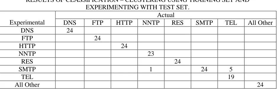
The results of the above experiment are given in Table 5. . It can be seen that a total of 6 vectors are misclassified (1 NNTP and 5 TELNET). Hence, we get 96.88% accuracy in estimating the application to which a particular packet size distribution belongs.
TABLE 5
RESULTS OF CLASSIFICATION – CLUSTERING USING TRAINING SET AND EXPERIMENTING WITH TEST SET.
Actual
Experimental DNS FTP HTTP NNTP RES SMTP TEL All Other
DNS 24
FTP 24
HTTP 24
NNTP 23
RES 24
SMTP 1 24 5
TEL 19
All Other 24
We then repeat the same experiment in a reverse manner, i.e. we form the clusters using the test data set, and test using the training data set. The results of that are given in Table 6. Here, we see that 9 vectors are misclassified, i.e. we get 95.31% accuracy.
TABLE 6
RESULTS OF REVERSE CLASSIFICATION – CLUSTERING USING TEST SET AND EXPERIMENTING WITH TRAINING SET.
Actual
Experimental DNS FTP HTTP NNTP RES SMTP TEL All Other
DNS 24
FTP 22
HTTP 1 24
NNTP 1 23
RES 18
SMTP 1 6 24
TEL 24
All Other 24
F. Classification of New Data
We collected new data from the North Carolina State University backbone network to validate the classification methodology that was developed using the old data. Like the old traces, the new ones also had roughly 500,000 packets in each file. We formed two data-sets out of the traces – Training set and Test set, each having 24 files in them, similar to the old data-sets. The difference between the two was that in the new data we did not have RESERVED traffic, and the mix of applications was different, i.e. the percentage contribution of each application differed. Using the same packet size distribution and classification algorithm, the new data sets were put through the same classification process.
The results of forming clusters using the new Training data-set and classifying the new Test data-set are given in Table 7, and those of the reverse process in Table 8. We see that we get a respective classification efficiency of 91.67% and 87.5%.
TABLE 7
RESULTS OF CLASSIFICATION OF NEW DATA – CLUSTERING USING TRAINING SET AND EXPERIMENTING WITH TEST SET.
Actual
Experimental DNS FTP HTTP NNTP SMTP TEL All Other
DNS 24 11
FTP 24 1
HTTP 24 1
NNTP 22
SMTP 24
TEL 12
TABLE 8
RESULTS OF REVERSE CLASSIFICATION OF NEW DATA – CLUSTERING USING TEST SET AND EXPERIMENTING WITH TRAINING SET.
Actual
Experimental DNS FTP HTTP NNTP SMTP TEL All Other
DNS 24
FTP 23
HTTP 24 2
NNTP 20
SMTP 20 7
TEL 12
All Other 1 2 4 5 24
IV. CONCLUSION AND FUTURE WORK
We saw that using clustering algorithms, we are able to classify major applications of Internet traffic. From that, it can be concluded that classification of Internet traffic using the features that are intrinsic characteristics of the packets, and features that cannot be spoofed so easily, is possible. This gives a completely new perspective of ‘implicit’ classification for differentiated services.
The work on classification in this manner is yet in its embryonic stage. The algorithms used have to be refined to attain greater accuracy and efficiency. Also, it should be noted that we used ‘pure’ traffic for classification, i.e. the test vectors were purely that of the application, while the Internet traffic is a mixture of all applications. The further refinement in the algorithms should support classification in these practical conditions. The future work will have to distinctly identify the time-critical applications and include them in the study.
Along with this refinement of algorithm work, a parallel study is to be done of estimation and prediction, as is mentioned in the long-term goals of this project. Identifying the characteristics of applications that can help classify them is only the first step in the mixture estimation problem. And after estimation, we have to be able to predict the traffic mix for successive times. This may involve training the system using neural networks and similar adaptive techniques. With the estimation and prediction problems resolved, methods for using this information in routers and schedulers can be developed.
REFERENCES
[1]. Mika Ilvesmaki, Marko Luoma, Raimo Kantola: Flow classification schemes in traffic-based multilayer IP switching – comparison between conventional and neural approach, Computer communications 21 (1998), pp. 1184-1194.
[2]. Fulu Li, Nabil Seddigh, Biswajit Nandy, Diego Malute: An empirical study of today’s Internet traffic for Differentiated Services IP QoS, Proceedings of ISCC 2000.
[3]. K. Glaffy, G. Miller, K. Thompson: The Nature of the Beast: Recent traffic measurements from an Internet Backbone, Proceedings of INET ’98, June 1998.
[4]. Assigned Port Numbers, http://www.iana.org/
[5]. Dan Decasper, Zubin Dittia, Guru Parulkar, Bernhard Plattner: Router Plugins: A software architecture for next-generation routers, IEEE/ACM Transactions on Networking, Vol. 8, No. 1, February 2000.
[7]. Mary L. Bailey, Burra Gopal, Michael A. Pagels, Larry L. Peterson, Prasenjit Sarkar: PathFinder: A pattern-based packet classifier, Proceedings of the First Symposium on Operating Systems Design and Implementation, pp. 115-123, November 1994.
[8]. S. Blake, D. Black, M. Carlson, E. Davies, Z. Wang, W. Wiess: An Architecture for Differentiated Services, RFC 2475.