ABSTRACT
SIDDIQUI, NASIR UDDIN. Methods For Calibrating and Validating Stochastic Micro-Simulation Traffic Models. (Under the direction of Dr. Nagui M. Rouphail.)
The purpose of this research was to propose a multistage framework for the
calibration and validation of the traffic simulation models and present results of a
calibration and validation experience using CORSIM model for a network of urban
streets. The study proposed a series of logical, sequential steps for the calibration and
validation of micro-simulation traffic models. The test bed used for the study is an
important network of traffic signals in the city of Chicago, Illinois. The internal network
consisting of twelve nodes at the core of the network served as the main focus of the
calibration and validation experience for this study. Base data was collected using video
and manual counts for extended AM and PM peak periods.
Two methods for determining the number of model repetitions were proposed: a)
use of statistical formula based on desired confidence interval and degree of confidence,
and b) model-based sensitivity test which examines the number of outlier runs and the
variability (distribution) in the model output from running sets of 25, 50, and 100 model
runs. The study showed that both methods compliment each other in arriving at the
required number of model repetitions.
Automation processes using the REXX code was used for extracting the required
model outputs and perform analysis of repetitive and multiple model runs during the
consisted of four distinct stages: a) error checking, b) calibration of input parameters for
capacity and demand (throughput comparisons), c) model tuning, and d) demand
adjustment. The study showed that the concept of split links in modeling long term
blockages by curb side parked vehicles proved to be more useful as compared to the
NETSIM record types for long term events and parking activity. The study also showed
the use of ‘In’ and ‘Out’ throughput volumes as an efficient and effective tool in
calibration of micro-simulation models for urban street networks.
Outputs from the calibrated and ‘tuned’ model for 100 replications were used in
the model validation for test network. The research demonstrated the use of the mean
stop time per vehicle and its modified form – the mean stop time per stopped vehicle as
effective and efficient measures for use in validation of micro-simulation models.
Between the mean stop time per vehicle and the mean stop time per stopped vehicle, the
later proved to be more useful in the validation process primarily because it eliminates
the difference between the model and the real-world which is purely on the basis of
difference in the values of percent stops counts.
For the test network, nine alternative scenarios were used for the model validation
criteria in terms of the level of significance and the proportion of links using two-sample
t-test. The study showed that the answer to the question whether the model is valid is
dependant upon the satisfaction of the pre-defined criteria. The answer changes as the
The key contribution of this research is the development of a multistage
methodological framework for calibration and validation of micro-simulation traffic
models. The methodology is quick to set up and implement on traffic networks and can
be used beneficially by future analysts and researchers.
BIOGRAPHY
Nasir Siddiqui was born and raised in the port city of Karachi, Pakistan. He received his elementary and secondary school education in Karachi. After completing his higher secondary school diploma in pre-engineering science from Government National College, Karachi, he pursued his undergraduate studies in civil engineering at NED University of Engineering and Technology, Karachi, where he received his Bachelor of Science degree in civil engineering in 1982. Following graduation, he started his engineering career as a transportation engineer with Pakistan’s largest private sector consulting engineering firm, Engineering Consultants International with its head office located in Karachi, Pakistan.
During his career with Engineering Consultants International, Nasir worked on projects involving major traffic corridor studies in Karachi, and planning and designs of major highways in Pakistan and in Middle Eastern countries. In 1989, he joined the Louis Berger Associates (LBA)/Construction Control Services Corporation (CCSC), a US Joint Venture as a Senior Design Engineer and worked on the United States Agency for International Development (USAID) funded Rural Roads Improvement Project in the province of Sindh, Pakistan. Nasir worked with LBA/CCSC Joint Venture for one year until 1990.
Nasir re-joined Engineering Consultants International as a senior transportation engineer in 1990. During his career with Engineering Consultants International, he worked on projects involving economic and environmental feasibility studies, and planning and designs of highways and expressways in various parts of the country funded by the World Bank and the Asian Development Bank (ADB), Manila, Philippines. Between 1993 and 1998, Nasir headed the traffic engineering and transportation planning division of the firm as a Principal Engineer and provided consulting engineering services for a number of transportation projects including the M1 Motorway between Peshawar
iii Kyrghizstan (former Soviet Union), on a joint venture of Engineering Consultants International and Kyrghizstan Road Transport Corporation.
In September 1997, Nasir married Farzana (Shaikh) Siddiqui, with whom he has two children, five-year-old Faizan and two year old Samiyah.
Nasir received a fellowship for graduate degree studies in transportation engineering from the International Road Educational Foundation in 1998. He began his graduate studies towards a Masters of Science degree in civil engineering with major in transportation engineering at North Carolina State University, Raleigh, in 1999. Here Nasir also worked as a research assistant under Dr. Nagui M. Rouphail and Dr. Joseph E. Hummer in the Civil Engineering Department, while pursuing his graduate studies. This thesis completes the final requirement for this degree.
ACKNOWLEDGEMENT
I would first like to thank the thesis advisory committee members and professors at North Carolina State University, Dr. Nagui M. Rouphail, Dr. Joseph E. Hummer, and Dr. John R. Stone for their valuable support and encouragement throughout the course of this research. As my advisory committee chair, Dr. Nagui Rouphail always made time in providing technical expertise and guidance throughout the thesis process. His enthusiasm, insight, and fellowship provided an invaluable experience. This would not have been possible without him. Dr. Joseph Hummer and Dr. John Stone provided valuable support and guidance. Their involvement and helpful comments on the final document made this thesis a much better product.
I am also thankful to Dr. Alan Karr and Dr. Jerome Sacks of the National Institute of Statistical Sciences (NISS) for providing office support facilities during the model coding and calibration process and for supplying the videotapes that provided valuable field data for use in this research. This research originated from RTTRACS study carried out at NISS.
Thanks are also due to Dr. David Johnston, Director of Graduate Program at the Civil Engineering Department, and his administrative assistants Edna White, and Renee Howard for their cooperation and support during the entire course of graduate studies at North Carolina State University.
In addition, I would like to thank several current employees of the North Carolina Department of Transportation, including Nathan Phillips, James Dunlop, Terry Hopkins, and Teresa Becher. Your assistance, understanding, and flexibility regarding work hours were greatly appreciated.
v
Last, but certainly not least, I would like to thank my mother Surrayya Jabeen for her sincere love, encouragement, and affection, and my wife Farzana Siddiqui, who shared the pains and happiness during all this period, and for her endless love, encouragement, and undying support.
TABLE OF CONTENTS
Page
LIST OF TABLES .....ix
LIST OF FIGURES ....xiii
LIST OF ABBREVIATIONS ....xv
1. INTRODUCTION ...1
1.1 Problem Definition...1
1.2 Research Objective...2
1.3 Layout of Report ...3
1.4 Background ...4
2. LITERATURE REVIEW ...5
2.1 General ...5
2.2 Studies Focusing on Micro-Simulator CORSIM ...5
2.3 Studies Involving Assessment of Alternatives and Model Comparisons...10
2.4 CALTRANS Guidelines ...13
2.5 Summary of Literature Review ...15
3. METHODOLOGY... 18
3.1 General Approach ...18
3.2 Model Description...18
3.3 Methodology Applications...20
3.4 Coding Base Network ...26
3.4.1 Base Network ...26
3.4.2 Input Parameters ...28
3.4.3 Error Checking ...30
3.5 Model Calibration ...31
3.5.1 Number of Model repetitions ...31
3.5.2 Process Automation ...36
3.5.3 Simulation Period ...37
3.5.4 Calibration Parameters ...38
3.5.5 Calibration Performance Measures ...39
3.5.6 Visual Review...43
3.5.7 Quantitative Evaluation...44
vii
4. BASE DATA COLLECTION ...46
4.1 General ...46
4.2 Base Network ...46
4.2.1 Geometry ...47
4.2.2 Traffic Control Parameters ...47
4.3 May 2000 Counts ...49
4.3.1 Scope...49
4.3.2 Entry Demand Volumes ...51
4.3.3 Proportion of Heavy Vehicles...55
4.3.4 Video Data Reduction...55
5. CASE STUDY MODEL CALIBRATION AND VALIDATION...63
5.1 General ...63
5.2 Model Calibration ...63
5.2.1 Input Parameters ...65
5.2.2 Error Checking ...66
5.2.3 Simulation Period ...66
5.2.4 Measures of Effectivenes ...67
5.2.5 Calibration Targets ...68
5.2.6 Analysis of Results ...70
5.3 Model Validation...87
5.3.1 Measures of Effectiveness for Evaluation...87
5.3.2 Results of Evaluation ...90
5.3.3 Significance Tests ... 105
6. SUMMARY, CONCLUSIONS, AND RECOMMENDATIONS ...108
6.1 Summary ...108
6.2 Conclusions ...113
6.3 Recommendations for Future Research ...114
7. LIST OF REFERENCES ...116
8. APPENDICES ...118
Appendix A: Schematic Layout of Study Network ...118
Appendix B: Location of Video Stations...122
Appendix C: Summaries of Traffic Counts and Turning Proportion Counts ...124
Appendix D: Video Data Reduction ...128
ix
LIST OF TABLES
Table Page
2.1. Wisconsin DOT Model Calibration Criteria ... 14
2.2. Summary of Literature Review: Checklist of Studies Covering Various Aspects of Calibration and Validation of Micro-Simulation Models ...16 3.1. Minimum Repetitions to Obtain Desired Confidence Interval ... 32
3.2. Comparison of Total Queue Time (veh-hrs) from Different Number of Run Repetitions for Non-Calibrated Model (4-6 PM)... 35
4.1. RT-TRACS PM Base Signal Timing Plan... 48
4.2. Summary of Entry Demand Volumes during PM Peak Period... 52
4.3. Summary of Video Counts for Internal Links for PM Peak ... 58
4.4. Percent Stopped Vehicles Counts and Stopped Delay for PM Peak (4-5 PM) ... 61
4.5. Percent Stopped Vehicles Counts and Stopped Delay for PM Peak (5-6 PM) ... 61
5.1. Model Calibration Criteria ... 69
5.2 System-level MOE's for Calibrated Model; Cumulative for 2-hr period (4-6 PM) ... 79
5.3. System-level MOE's for Partially Calibrated Model (Unadjusted Demand and No Split Links on LaSalle; Cumulative for 2-hr period (4-6 PM) ... 81
5.4. Comparison of In & Out Total Throughput Volumes (4-6 PM); Field Vs. Model (Partially Calibrated Model with No adjustment in Demand and No split Links on LaSalle) ... 82
5.5. Comparison of In & Out Total Throughput Volumes (4-6 PM); Field Vs. Model (Calibrated Model with Adjusted Demand and Split Links on LaSalle) ... 82
5.6. Comparison of In & out Throughput Volumes (4-5 PM); Case p131a (Adjusted Demand Volumes; 2 & 3 Lanes links on LaSalle)... 84
5.7. Comparison of In & out Throughput Volumes (5-6 PM); Case p131a (Adjusted Demand Volumes; 2 & 3 Lanes links on LaSalle)... 84
5.8. Calibration Target Checks for the Internal Network... 86
5.9. Comparison of Link Trips and Stop Delay 4-5 PM ... 91
5.11. Comparison of Percent Stops and Stopped Vehicles Stop Delay 4-5 PM ... 99
5.12. Comparison of Percent Stops and Stopped Vehicles Stop Delay 5-6 PM ... 100
5.13. Comparison of Field and Model Validation MOE; p-values for two-sample t-test ... 106
5.14. Alternative Scenarios for Model Validation Criteria for Internal Network ... 107
APPENDIX TABLES: C.1. Summary of External Station Counts for PM Peak (4-6 PM)... 125
D.1. Summary of In and Out Video Counts for Internal Network for PM Peak Hours129 D.2. Summary of Link Trips by Turn Movement (4-6 PM) ... 130
D.3. In and Out Trips for Internal Network from Video Counts ... 131
D.4. Summary of Turn Percentages by Movements at Internal Nodes... 133
D.5. Summary of Counts by 5-Minute Intervals (4-6 PM); Ontario and Orleans ... 135
D.6. Summary of Counts by 5-Minute Intervals (4-6 PM); Franklin and Ontario ... 136
D.7. Summary of Counts by 5-Minute Intervals (4-6 PM); Wells and Ontario... 137
D.8. Summary of Counts by 5-Minute Intervals (4-6 PM); LaSalle and Ontario... 138
D.9. Summary of Counts by 5-Minute Intervals (4-6 PM); Orleans and Ohio... 139
D.10.Summary of Counts by 5-Minute Intervals (4-6 PM); Franklin and Ohio ... 140
D.11.Summary of Counts by 5-Minute Intervals (4-6 PM); Wells and Ohio... 141
D.12.Summary of Counts by 5-Minute Intervals (4-6 PM); LaSalle and Ohio... 142
D.13.Summary of Counts by 5-Minute Intervals (4-6 PM); Orleans and Grand ... 143
D.14.Summary of Counts by 5-Minute Intervals (4-6 PM); Franklin and Grand ... 144
D.15.Summary of Counts by 5-Minute Intervals (4-6 PM); Wells and Grand ... 145
D.16.Summary of Counts by 5-Minute Intervals (4-6 PM); LaSalle and Grand ... 146
D.17.Summary of Non-Stopping Vehicle Counts ... 147
D.18.Summary of Percent Stopped Vehicle Counts and Stopped Delay for PM Peak (4-5 PM) ... 148
D.19.Summary of Percent Stopped Vehicle Counts and Stopped Delay for PM Peak (5-6 PM) ... 148
xi E.1. Summary of System Level MOE’s for Uncalibrated Model (Case ‘p0622a’);
Cummulative for 2-hour Period (4-6 PM) for 100 Runs... 155
E.2. System Level MOE’s for Outlier Runs for Uncalibrated Model (Case ‘p0622a’); Cummulative for 2-hour Period (4-6 PM) for 100 Runs... 155
E.3. Summary of System Level MOE’s for Partially Calibrated Model (Case ‘p131r’); Cummulative for 2-hour Period (4-6 PM) for 100 Runs ... 157
E.4. System Level MOE’s for Outlier Runs for Partially Calibrated Model (Case ‘p131r’); Cummulative for 2-hour Period (4-6 PM) for 100 Runs ... 157
E.5. Summary of System Level MOE’s for Calibrated Model (Case ‘p131a’); Cummulative for 2-hour Period (4-6 PM) for 100 Runs... 159
E.6. In & out Throughput Volumes for Partially Calibrated Model (Case 'p131r'; Unadj. Demand Volumes and No Split links (All 3 Lanes) on LaSalle): Field versus CORSIM (4-5 PM)... 161
E.7. In & out Throughput Volumes for Partially Calibrated Model (Case 'p131r'; Unadj. Demand Volumes and No Split links (All 3 Lanes) on LaSalle): Field versus CORSIM (5-6 PM)... 161
F.1. Link Stop Time (sec/veh) for 4-5 PM; Calibrated Model (Case ‘bmf’) ... 163
F.2. Summary Statistics for Link Stop Time (sec/veh) for 4-5 PM; (Case ‘bmf’)... 164
F.3. Link Percent Stops (%) for 4-5 PM; Calibrated Model (Case ‘bmf’)... 165
F.4. Summary Statistics for Percent Stops (%) for 4-5 PM; (Case ‘bmf’)... 166
F.5. Link Stop Time per Stopped Vehicle (sec/veh) for 4-5 PM; Calibrated Model (Case ‘bmf’) ... 167
F.6. Summary Statistics for Link Stop Time per Stopped Vehicle (sec/veh) for 4-5 PM; (Case ‘bmf’) ... 168
F.7. Link Stop Time (sec/veh) for 5-6 PM; Calibrated Model (Case ‘bms’) ... 169
F.8. Summary Statistics for Link Stop Time (sec/veh) for 5-6 PM; (Case ‘bms’)... 170
F.9. Link Percent Stops (%) for 5-6 PM; Calibrated Model (Case ‘bms’)... 171
F.10. Summary Statistics for Percent Stops (%) for 5-6 PM; (Case ‘bms’)... 172
F.12. Summary Statistics for Link Stop Time per Stopped Vehicle (sec/veh)
for 5-6 PM; (Case ‘bms’) ... 174 F.13. Summary of Link Throughput Volumes (Vehicles) for 4-5 PM and 5-6 PM;
xiii
LIST OF FIGURES
Figure Page
3.1. Methodology Flowchart ... 22
3.2. Location Map of Study Network in Chicago ... 27
3.3. Test-Bed Network ... 28
3.4. Comparison of system Queue Time for 25, 50, and 100 Model Repetitions for the Non-Calibrated Model... 34
3.5. Number of Outlier Runs versus Number of Model Repetitions for Non-Calibrated Model ... 34
3.5. Number of Outlier Runs versus Number of Model Repetitions for Partially Calibrated Model... 36
4.1. Location of Video and Manual Count Stations... 50
4.2. Variation of Northbound Input Volumes during PM Peak ... 54
4.3. Variation of Southbound Input Volumes during PM Peak ... 54
4.4. Variation of Westbound Input Volumes during PM Peak ... 55
4.5. CORSIM Representation of Test Network – Link & Node Diagram ... 57
4.6. Average Stopped Delay for PM Peak ... 62
5.1. Snapshot of internal network for partially calibrated model at 16:40 PM: Spillback on northbound Franklin at Grand just beginning to appear ... 72
5.2. Snapshot of internal network for partially calibrated model at 17:000 PM: Traffic gridlock extends to large portion of network on LaSalle, Grand, Ohio, and Orleans streets ... 72
5.3. Split links on LaSalle with 2 & 3 Lanes; Between Ontario & Erie (Top) and between Illinois & Grand (Bottom)... 76
5.4 Snapshot of Thru and Left Turn Split Links on Northbound Orleans between Ohio and Ontario; Vehicles on upstream link 9->5 positioning themselves for turn maneuvers on the downstream split link 5->1 ... 77
5.5. System Queue Time Distribution for Calibrated Model ... 80
5.7. Throughput Comparisons for Entry and Exit Links of Internal Network –
Field Vs. Model (4-5 PM) ... 85
5.8. Throughput Comparisons for Entry and Exit Links of Internal Network – Field Vs. Model (5-6 PM) ... 85
5.9. Link Stop Delay Comparison - CORSIM versus Field... 96
5.10. Link Stop Delay per Stopped Vehicle Comparison - CORSIM versus Field ... 103
APPENDIX FIGURES: A.1. Location Map of Study Network in... 119
A.2. Test-Bed Network Showing Location of Video and Manual Count Stations ... 120
A.3. Schematic Layout of Internal Network ... 121
C.1. Variation of Southbound Input Volumes, Stations E1 to E7 ... 126
C.2. Variation of Westbound Input Volumes on Ontario and Grand ... 126
C.3. Variation of Northbound Input Volumes on LaSalle, Franklin, and Orleans ... 127
E.1. System Queue Time for Non-Calibrated Model (Case 'p622a') for 100 Runs; 4-6 PM... 156
E.2. Comparison of System Queue Time for Non-Calibrated Model (Case 'p622a') for 100, 50, and 25 Runs; 4-6 PM ... 156
E.3. System Queue Time for Partially Calibrated Model (Case 'p131r') for 100 Runs; 4-6 PM... 158
E.4. Comparison of System Queue Time for Partially Calibrated Model (Case 'p622a') for 100, 50, and 25 Runs; 4-6 PM ... 158
xv
LIST OF ABBREVIATIONS
Symbol Description
ADB Asian Development Bank
ANOVA Analysis of Variance
CALTRANS California Department of Transportation
CDOT Chicago Department of Transportation
CI Confidence Interval for Mean Value in a Statistical Distribution EB Eastbound
FHWA Federal Highway Administration
hr, hrs Hour, Hours
ITS Intelligent Transportation System
mi Mile(s) min Minute(s)
N/A, n/a Not Applicable
NB Northbound
NC North Carolina
NCSU North Carolina State University
NISS National Institute of Statistical Sciences
OD Origin & Destination
PI Performance Index
RNS Random Number Seed(s)
RT Record Type
RTOR Right-Turn-On-Red RT-TRACS Real Time Traffic Control System
S.D., s.d Standard Deviation
SB Southbound Std. Standard sec Second(s)
TWLTL Two-Way Left-turn Lane
USAID United States Agency for International Development
USDOT United States Department of Transportation
UTC Urban Transportation Center
veh Vehicle(s)
VMT Vehicle Miles of Travel
Vs., vs. Versus
WB Westbound
CHAPTER 1
INTRODUCTION
1.1 Problem Definition
Traffic system operation is characterized by the flow of mobile elements (users and vehicles) through facilities (roadways and control devices). The flow of the mobile elements is a complex interactive process. This process is a function of facility design, user objectives, perceptions and reaction of drivers, and vehicle dynamics. A traffic system software is a symbolic software model for conducting experiments on a traffic system. The purpose of the experiments is to design and modify the facilities to optimize safety and efficiency of traffic flow.
Since the emergence of Intelligent Transportation Systems in the 1990s, simulation has become an invaluable tool for evaluating the ITS strategies whether they relate to a system of freeways or to a complex urban road network. While considerable research efforts have been devoted to the development of traffic simulation model, validation, which is an integral part of the ‘model development life cycle’, has not received enough attention (Rao et al., 1998) (1).
Calibration is a mathematical process to identify the global and link specific parameters for driver behavior and vehicle operation that cause the simulation model to best reproduce the observed real-world behavior for local conditions. Calibration is performed locally by the analyst for each individual application of the simulation model to the real-world network. Validation is the act of determining whether a simulation model reasonably represents or approximates the real system for its intended use (Fishman and Kiviat 1968, Sargent 1982, Law and Kelton 1991).
2
being caught in a never-ending circular process where fixing one problem may result in
popping of a new one somewhere else (CALTRANS / Dowling et. al., 2002) (13)
.
The validation of the computer simulation models is a crucial element in assessing their value for making transportation policy, planning, and operational decisions. The need to develop a (validation) framework is compelling, even urgent. The use of computer models by transportation engineers and planners is growing; costs of poor decisions is escalating; and increasing computer power, for both computation and data collection, is magnifying the scale of the issues (Sacks et al., 2001) (2).
Examples of micro-simulation models in use are: Aimsum, CORSIM, Paramics, Simtraffic, Transmodeller, VISSIM, WATSIM, etc. They stochastically model individual vehicle movements as a function of time and space. Most of the simulation models developed in the traffic engineering community do not have guidelines for validation. For instance, it is usually left to the users to choose a number of parameters to vary in order to study the way the simulation behaves, and to understand the significance of any difference between observed measures from the real world and simulated measures of effectiveness (Rao et al., 1998) (1). These models often do not include any specifications to deal with the parameter adjustments and interpreting those differences.
1.2 Research Objectives
The purpose of this study is to propose a multistage framework for the calibration and validation of the traffic simulation models and present results of a validation experience on an urban street network. The research effort also focused on laying out a set of key issues involved with the complex processes of calibration and validation of the micro-simulation traffic models. The microscopic simulation model used for this study is
CORSIM (CORridor SIMulation) (9), which is the most widely used model in the United
The objectives of the research effort are manifold:
Understand the functioning of the microsimulator CORSIM, specifically NETSIM as applicable to urban street networks
Propose a step by step methodology for calibration and validation of microsimulation models
Demonstrate the methodology by presenting the results of a calibration and validation experience on a case study network
Layout a set of key issues involved, and
Present findings and conclusions of the case study calibration and validation
The model validation was performed as part of the application of the micro-simulator CORSIM in assessing the signal timing plans for the street network in downtown Chicago.
For the case study network, this research only used the PM peak period (4-6 PM) data for calibration and validation of the base network because of the constraint on time and resources, though the base data was collected using manual and video counts for the AM and PM peak periods. The CORSIM version 4.32 was used for the case study calibration and validation. The case study network consisted of 31 intersections formed by a network of arterial streets in Chicago, Illinois. The research effort focused on calibrating and validating the internal network consisting of twelve signalized intersections at the core of the study network.
1.3 Layout of Document
4 methodology as applied to the calibration and validation processes of the test bed. Base data collection and network coding is described in Chapter 4. Chapter 5 presents the results of the model calibration and validation experience for the test bed. Chapter 6 summarizes the study findings and conclusions and includes recommendations for future research. Chapter 7 presents a list of references to literature cited in this document. Appendices are included at the end of the document.
1.4 Background
CHAPTER 2
LITERATURE REVIEW
2.1 General
The purpose of the literature review was to conduct a thorough review of the past research involving calibration and validation of micro-simulation traffic models, and other studies involving the use of such models in the traffic-engineering field. Such a review was useful in providing the knowledge that already exists in the field and in determining the gaps in the past research in regards to the methods and techniques of calibration and validation of micro-simulation models.
The main focus of the literature review were studies dealing with the micro-simulator CORSIM (CORridor SIMulation) (9), which is the most widely used model in the United States for simulation of freeway and arterial networks as well as evaluation of these systems. The past research studies on micro-simulation models can be broadly classified in two categories: those focusing on micro-simulation models itself, addressing the elements of accuracy and variability in the simulation model output, and those involving micro-simulation models in assessment of alternatives and comparison of these models among themselves. The second category also includes studies that assessed alternatives as well as the micro-simulation model itself. In addition to the studies falling in the above two categories, a review of the guidelines for application of traffic micro-simulation models prepared by Dowlings et al. (13) for the California Department of Transportation (CALTRANS) is also presented later in the chapter.
2.2 Studies Focusing on Micro-Simulator CORSIM
6 Gafarian and Halati (3) assessed the efficacy of statistical method through the usage of Monte Carlo experiments. They discussed two different methods of running NETSIM (single, long run or multiple independent runs). The findings of the paper reveal that the method using multiple independent runs may be applied to the estimation of parameters. Also noted was the existence of an auto and cross-correlation amongst the NETSIM MOE's. Because of these correlations the usage of a single, long NETSIM run to develop a confidence interval was not recommended. Gafarian and Halati (3) suggested the extension of the developed method to the comparison of NETSIM outputs with field observations for simulation validation studies.
Benekohal and Abu-Lebdah (4) were among the first researchers who focused primarily on the NETSIM output and dealt exclusively with the issue of variability of traffic simulation outputs. They analyzed the variability of NETSIM outputs at three different levels of aggregation i.e. network level, link level, and intersection level, using the batch means method and the replication method. Since NETSIM reports cumulative MOE outputs for a given interval rather than the individual interval MOE values, the outputs from the batch means method are correlated (auto and cross-correlation). For correcting the problem of correlation in batch means method, Benekohal and Abu-Lebdah (4) suggested the use of a proposed interval calculation (PIC) method. In the PIC method, vehicle trips and phase failures are computed by finding differences between successive batches of time intervals. Similarly delays and speeds are computed using simple mathematical relationships. The study examined various measures of effectiveness outputs from NETSIM for a base and more heavily congested case using the batch means (BM/PIC) method and replication method. The replication method was comprised of twenty-four 10-minute NETSIM simulations; each with a different random number seeds (RNS). The batch method consisted of a single four-hour NETSIM run with intermediate results calculated every 10 minutes. The authors noted two key findings from the study:
consequently producing lower vehicle delays and higher average speeds. The variability of the batch means method output tends to be higher than the replication method.
Benekohal and Abu-Lebdah (4) also suggested approaches to determine the number of runs needed for the replication method and the batch size and length for the batch means method. The authors noted the consistency of their findings with the study conducted by Gafarian and Halati (3) regarding the use of the batch method in building confidence interval and caution the NETSIM user about the element of auto and cross-correlation in the NETSIM direct output. Finally, they recommended a comprehensive study dealing with the sensitivity and output variability of NETSIM.
8 The K-S test can be employed to test whether the values from the real world and those from the simulation are from the same distribution and is especially useful in comparing the correlated MOE distributions (e.g. speed versus headway) between the real world and the model. Using the mathematical expression from Press et al. (1992) for calculating the probability of the K-S statistic (D) being greater than a pre-defined level of significance (d), they included a step-wise procedure for conducting a two-dimensional two-sample K-S test between the real world and the simulation.
Rao et al. (1) presented results of a validation experience by applying the proposed validation framework on a one-directional arterial link between two signalized intersections using the microscopic simulation model CORSIM. They collected speed and headway data on five platoons along the arterial link and used the real-world data for running ten independent simulations for each platoon using CORSIM. They chose speed and headway as the validation MOE’s for the test case. For the first level of operational validation, they performed a two-sample t-test for each platoon by comparing the p-values obtained versus a pre-defined level of significance of 0.10. Based on the results obtained from the two-sample t-test, they found that the model was valid at the pre-defined level of significance and the chosen MOE’s for all the real world data sets. For the second level of operational validation, they chose speed and headway as the MOE pair for conducting the K-S two-dimensional two-sample test. Based on the results of the K-S test they found the model to be invalid at the second level of the operational validation. They concluded that validation was not a binary decision, but rather a decision based on the model’s intended use. The results from their validation experience demonstrated the necessity and advantages of the proposed validation procedure.
assessment of signal-timing plans on a street network in Chicago. The street network used in the study by Sacks et al. was part of the RTTRACS network and is the same network as used in this research for demonstration of a calibration and validation methodology. Sacks et al. used stop time per vehicle (STV) and stop time per stopped vehicles (STVS) as the validation MOE’s and performed comparison between the field and CORSIM output for selected links in the AM and PM peak hours. They also examined CORSIM for the degree of variability (over time) characteristic of the field data by comparing the field time series of throughputs with the one produced by the model. They defined the time series variation function as being equal to the sum of squares of differences in the subsequent intervals divided by the total number of time intervals. For a time series of 24 time points represented by 24 dual-cycle intervals (each 150 seconds) in a 60-minute period, the mathematical expression for the variation function given by Sacks et al. is given below:
t=1 23
∑[Y(t+1) – Y(t)]
Variation fn =
23
Where V(t) represents throughput during time interval t. Based on the comparison for selected links, they found the CORSIM variability to be close to that of field.
10
2.3 Studies Involving Assessment of Alternatives and Model Comparisons
Rouphail et al. (5) used TRAF-NETSIM for the validation of a generalized delay model, which was later incorporated in a 1997 update of the Highway Capacity Manual
(14), for vehicle-actuated signals. They did a simulation study involving an at-grade
intersection of two streets with near ideal traffic and geometry and a vehicle-actuated traffic control. They carried out a total of 640 NETSIM runs with different levels of traffic volumes on the major and minor streets and four different vehicle-actuated signal designs. They compared NETSIM delays with the generalized model delays. Also, comparisons were made between actual field-measured delays and the generalized model delays. They observed that the delays estimated by the generalized delay model were comparable with the delays estimated by NETSIM. The data compared favorably for degrees of saturation of 0.8 and lower. However, for higher degrees of saturation the generalized delay model produced delays that were higher than NETSIM. Rouphail et al.
(5) did not compare the NETSIM delays directly with the field-measured delays.
However, they compared their generalized model delays with the field-measured delays and found that the results were comparable.
Engelbrecht, Fambro, Rouphail, and Barkawi (6) used TRAF-NETSIM for the validation of a generalized delay model (incorporated in HCM 1997 update) for oversaturated conditions. They used the microscopic simulation model because of the practical difficulties associated with the measurement of oversaturation delay in the field. The study was designed to cover as much of the domain of oversaturated operations as possible. To speed up the simulation process and analysis of the outputs, Engelbrecht et al. (6) developed a computer program to generate random numbers, generate input files, run NETSIM, read output files and tabulate results. They noted that a stochastic microscopic simulation model, such as TRAF-NETSIM, yields many advantages over field surveys:
Using simulation is much quicker because simulation runs faster than the real time.
TRAF-NETSIM uses path-trace method to estimate overall delay. If field surveys are done, overall delay has to be estimated from stopped delay, introducing some error.
Simulation generates delay data under conditions that can be controlled by the analyst. Scenarios can, therefore, be selected to include the conditions under which the model will normally be used.
Based on the results from NETSIM simulation runs, Engelbrecht et al. (6) found that a good correlation existed between the estimated (predicted) delays and simulated delays. They used the outputs from NETSIM to investigate the variability in simulated overall delays and developed an equation to predict the standard deviation of oversaturated delay estimates.
Reid and Hummer (7) used NETSIM to compare two unconventional arterial designs with the conventional the two-way left-turn lane (TWLTL) arterial design with the purpose of testing the potential of alternative designs to provide an overall reduction in system travel times and other critical traffic operations measures of effectiveness (MOE’s). They carried out a traffic simulation study using a median U-turn design, a super-street design, and a traditional TWLTL design, involving four different time periods; AM peak, Noon Peak, Mid-day Peak, and PM Peak. Within each time period, the authors employed four different volume scenarios. Reid and Hummer (7) used SYNCHRO (11) to formulate the signal timing and offsets for each geometric alternative and output the results to NETSIM for running simulations. The experiment had 144 half-hour NETSIM runs in a full factorial design with three replications. The three measures of effectiveness used were system travel time, average number of stops, and the average speeds for the network. They carried out an analysis of variance (ANOVA) to test the significance of results with respect to geometry.
Park et al. (8) used CORSIM (NETSIM) to evaluate the reliability of TRANSYT-7F
(10) optimization strategies. The test bed used for this strategy was a Chicago street
2.4 CALTRANS Guidelines
Dowlings et al. (13) prepared guidelines for the application of traffic micro-simulation software to transportation project planning and development in a 2002 manual for the California Department of Transportation (CALTRANS). The emphasis of the manual was on training CALTRANS personnel on how to apply micro-simulation in combination with or in parallel with other software tools to evaluate the traffic operations of project alternatives.
The CALTRANS manual and its associated training course focused on the steps leading up to operation of the micro-simulation software and the steps after application of the software. In addition to explaining the general characteristics of micro-simulation models and the processes involved, the manual describes steps in data preparation and error checking. It provides guidance on the collection and preparation of the data sets needed to develop a micro-simulation model. The manual describes four stages of model calibration process, namely error-checking, calibration for capacity, calibration for demand, and overall review. The manual includes calibration targets developed by the Wisconsin Department of Transportation (15) based on guidelines developed in the United
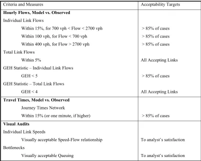
14 Table 2.1: Wisconsin DOT Model Calibration Criteria
Criteria and Measures Acceptability Targets
Hourly Flows, Model vs. Observed Individual Link Flows
Within 15%, for 700 vph < Flow < 2700 vph Within 100 vph, for Flow < 700 vph Within 400 vph, for Flow > 2700 vph Total Link Flows
Within 5%
GEH Statistic – Individual Link Flows GEH < 5
GEH Statistic – Total Link Flows GEH < 4
> 85% of cases > 85% of cases > 85% of cases
All Accepting Links
> 85% of cases
All Accepting Links
Travel Times, Model vs. Observed Journey Times Network
Within 15% (or one minute, if higher) > 85% of cases
Visual Audits Individual Link Speeds
Visually acceptable Speed-Flow relationship Bottlenecks
Visually acceptable Queuing
To analyst’s satisfaction
To analyst’s satisfaction
Source: FREEWAY SYSTEM OPERATIONAL ASSESSMENT, Technical Report I-33, Paramics Calibration & Validation Guidelines, DRAFT, Wisconsin Department of Transportation, District 2, June 2002(15)
The GEH statistic is computed as follows:
(V-F)
GEH =
√ (V+F)/2 Where,
GEH = the statistic
V = Model estimated directional hourly volume at a location F = Directional hourly count observed at a location
Finally the manual provides guidance on the analysis, and interpretation of micro-simulation model output. These guidelines include selection of key summary statistics, summarizing the key statistics, correction of biases in results, interpretation of animation and numerical outputs, and hypothesis testing of alternatives.
2.5 Summary of Literature Review
A review of the past research studies presented above shows that while different researchers focused on different aspects of validation of micro-simulation models and the elements of variability and uncertainty in the model output, a comprehensive study presenting a methodology covering the broad spectrum of calibration and validation of micro-simulation models seems to be missing so far.
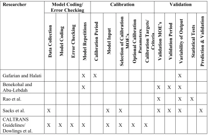
16 Table 2.2: Summary of Literature Review: Checklist of Studies Covering Various Aspects of
Calibration and Validation of Micro-Simulation Models
Model Coding/ Error Checking
Calibration Validation Researcher
Data Collection Model Coding Error Checking Model Repetitions Calibration Period Model Input
Selectio n o f Ca libra tio n MOE ’s Opti onal Cal ib rati on Parameters Calibration Targets/ Criteria Va lida tio n MOE’s Va lida tio n Perio d Va ria bility o f Output Sta tistica l Tests Predictio n & Va lida tio n
Gafarian and Halati X X X
Benekohal and
Abu-Lebdah X X X X
Rao et al. X X X
Sacks et al. X X X X X X X CALTRANS
Guidelines/
Dowlings et al. X X X X X X X X
The research studies in the second category involving micro-simulation models in assessment of alternatives and comparison of these models, although did not deal directly with the validation of micro-simulation models but some of them indirectly did. For example, Rouphail et al. validated the estimated delays from their generalized delay model with field-measured delays and then performed comparisons with the NETSIM delays. Other studies included methods and statistical tests in the evaluation of micro-simulation outputs while assessing the alternatives or performing comparisons among different models.
and will implement the proposed methodology on a test case of urban street network. As part of the proposed methodology and its implementation on a case study network, the research effort will also lay out a set of key issues involved with the complex processes of calibration and validation of these models. The microscopic simulation model CORSIM (9) will serve as the test-bed for the case study network as it is the most widely
as evaluation of these systems. Some of those methods included in the past research used model in the United States for simulation of freeway and arterial networks as well
18
CHAPTER 3
METHODOLOGY
3.1 General Approach
This chapter describes the methodology adopted for the calibration, evaluation
and validation of the traffic simulation model used for this research. The microscopic
simulation model used for this study is CORSIM, which is the most widely used model in
the United States for simulation of freeway and arterial networks as well as evaluation of
these systems. The test bed used for the study is an important network of traffic signals in
the city of Chicago, Illinois. A description of the simulation model and the methodology
flowchart are presented in the sections that follow. The detailed evaluation of the
simulation model consists of the following three distinct phases:
• Base Model Coding
• Model calibration and tuning
• Evaluation and Validation
A description of the methodology adopted for each of the above three phases of
study is presented later in this chapter.
3.2 Model Description
CORSIM is a stochastic and microscopic simulation model of urban traffic
developed by FHWA (9). CORSIM is a combination of two component models namely
NETSIM and FRESIM for surface street network and freeway network respectively.
CORSIM uses the concept of links and nodes to define the roadway network. The
network that represents the traffic environment can be divided into sub networks, which
interface with one another. The user has total control over partitioning the analysis
network into its component sub networks. NETSIM applies interval-based simulation to
time step, the step being equal to one second. Each variable control device and each event
are updated every time step. Up to nine different vehicle categories can be specified. A
‘driver behavioral characteristic’ is assigned to each individual vehicle and turn
movements are assigned stochastically, as are free-flow speeds, queue discharge
headways, and other behavioral attributes. As a result, each vehicle’s behavior can be
simulated in a manner reflecting real-world processes.
CORSIM is widely recognized throughout the literature as the standard by which
all other signal timing and evaluation programs are judged. Variation of this model has
been used in the U.S for over thirty years. Extensive testing has been done on the
CORSIM program and several modifications have been made throughout the years to
increase the program’s accuracy. Unlike the TRANSYT-7F (10) and SYNCHRO (11)
programs, CORSIM does not generate or optimize traffic signal plans and is primarily
used as an evaluation tool to study the performance of various plans and systems.
For the CORSIM model, the input stream consists of a sequence of ‘record types’, which are also called ‘cards’ or ‘card types’. Network data are entered into the program through the creation of a text file with various card types. This text file also known as ‘.trf’ file is created either manually or by using an interactive traffic network data editor called ‘ITRAF’, which has a graphical interface developed to simplify the task of creating data files as inputs to CORSIM. But ITRAF is still a prototype and its development is an ongoing process. It is still considered somewhat difficult for the novice user. Once the input file is created, the network can be simulated and the reader has the option to either view the output or view an animation of simulated traffic network in the graphical output editor TRAFVU.
20
operations or “snapshots” of network conditions at specified time intervals are required. For this study CORSIM version 4.32 was utilized. A description of the test network coding is described in the section that follows.
3.3 Methodology Application
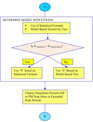
Figure 3.1 presents a step by step methodology for model calibration and
validation in the form of a flow chart. As shown in the figure, the first step in the
calibration of a microsimulation model is to identify the project purpose, scope and
approach. This is followed by the data collection stage which includes input data for the
base model, calibration data, validation data, and future demands. Input data for the base
model consists of network geometry, traffic controls, and existing demands. Calibration
data consists of measures of capacity and system performance such as throughputs,
headways, speeds, travel times, delays, and queues. Validation data consists of the
selected output data such as the throughputs, stop delays, percent stops, and travel times
used as the validation measures of effectiveness (MOE’s). Future demands are the
forecasts obtained from the regional travel demand model or those from the trend line
forecasts based on historic data. Data collection for the base model is described in
Chapter 4 of this document.
As a next step in model calibration, the base model is coded by entering the input
data on geometry, controls, and demands into the microsimulator. This is followed by a
thorough error checking procedure to ensure that the input data is entered correctly in the
model. Error checking is a repetitive process that involves various tests of the coded
network. This involves repetitive model runs at low volumes and performing visual
reviews of the model animations to identify these errors. Once the errors are eliminated
and any inconsistencies in the network coding are removed, we have a model that is
As shown in Figure 3.1, the next step in model calibration is to determine the
number of model repetitions using the statistical tools or the model based sensitivity tests.
This is followed by the selection of the simulation period for model calibration.
The model calibration process involves a sequence of steps, computations and
criteria for determining if the simulation model is reasonably consistent with the real
world. The steps involved in the process include choosing the calibration parameters,
choosing the performance indices and MOE’s, and running multiple model runs to
calibrate one or more calibration parameters. The multiple model runs are executed and
model outputs are extracted using the process automation. This is followed by visual
review of the animation product and quantitative evaluation of various performance
measures. If the visual and quantitative criteria are not satisfied, the process is repeated
by modifying the calibration parameter so as to satisfy the visual and quantitative checks.
Where the model performance in some specific links deviates substantially from field,
some of the link attributes may be adjusted so as to best match the real world. Once the
selected optional input parameters are calibrated by satisfying the visual and quantitative
criteria, the next step is to perform checks against the calibration targets. This involves
comparison of the individual and total link flows between the model and the field values.
If these values are not within the pre-defined range or target, the entry demands are
adjusted so as to best match the observed throughputs for the individual links and at the
network level. The steps of base model coding and model calibration are discussed in
detail in the sections that follow.
After the model is calibrated, the next sequence of steps belongs to the model
validation process. The purpose of model validation is to determine whether a simulation
model reasonably represents or approximates the real system for its intended use (Rao et
al., 1998) (1). The steps of validation methodology adopted for the test bed are discussed
20
A DATA COLLECTION:
Input Data For Model (Geometry, Controls, Existing Demands)
Calibration Data (Performance Data Such As Throughput, Speed, Queues, Headways, Driver Behavior
Characteristics Etc.)
Validation Data (Selected Output Data Such As Throughput, Stop Time, Percent Stops, Travel Time)
Future Demands (Turn Volumes, OD Table)
Identification of Project Purpose, Scope, and Approach
BASE MODEL CODING(1)
Model Coding (Input Geometry, Controls, Demands)
BASE MODEL CODING (2):
ERROR
CHECKING
Yes
No
Review Link Attributes Review Demands
Error Check? Run/Re-Run Model at Low Volumes
Fix Errors
Perform Visual Review
Trace Selected Vehicles through Network
Figure 3.1 (Continued) A
DETERMINE MODEL REPETITIONS:
Use of Statistical Formula
Model Based Sensitivity Test
Is N Statistical > N Model Based?
Yes No
Use ‘N’ based on
Statistical Formula Use ‘N’ Based on Model Based Test
Choose Simulation Period (AM or PM Peak Hour or Extended Peak Period)
22
Figure 3.1 (Continued) B
C MODEL CALIBRATION:
Choose Calibration Parameters
Choose Performance Indices or MOE’s
Process Automation: Run/Re-Run Multiple Model Runs & Extract Outputs
No Is Quantitative
Criteria Satisfied?
Visual Review (Median, Quartile, or Outlier Runs)
Quantitative Evaluation (System MOE’s; Queue Time, Stop Time, Throughput)
Is Visual Criteria Satisfied?
Do Calibration Targets Meet? (Statistical Tests)
No
Yes
Calibrated Model No
Calibrate One or More Calibration Parameters
Model Tuning (Link Specific Attributes)
Adjust Demands (Entry Volumes, Turn Percentages)
Figure 3.1 (Continued) C
MODEL VALIDATION:
Select Validation Period
Select Validation MOE’s
Select Links and/or Corridors for Evaluation
PROCESS AUTOMATION: Run Multiple Model Runs and Extract Outputs
QUANTITATIVE EVALUATION:
Compute Statistical Measures of MOE’s
Field vs. Model Comparisons (Means, Confidence Intervals)
Plots of MOE Distribution vs. Field Value
Select Validation Targets (Confidence Level, Percent of Links Satisfying Criteria)
STATISTICAL TESTS:
Probability of Error (Model <or> Field at Pre-defined Conf. Level)
Do Validation Targets Meet?
Model is Valid for the Predefined Criteria
Yes Model is Invalid for
the Predefined Criteria No
26
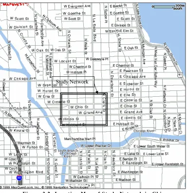
3.4 Coding Base Network
3.4.1 Base Network
The base network is in downtown Chicago (Illinois) consisting of 31 intersections
and is bound by Clark Street in east, Erie Street in north, Illinois Street in south, and
Kingsbury Street in west. The network is part of the RT-TRACS study conducted with
the cooperation of Chicago Department of Transportation (CDOT). The ultimate goal of
the RT-TRACS study is to optimize the signal plans for a network more extensive than
the one below. The focus of study is the internal network consisting of 12 intersections
formed by 3 east-west streets, namely Ontario, Ohio, and Grand, and 4 north-south
streets, namely LaSalle, Wells, Franklin, and Orleans. Figure 3.2 shows location map of
the project network and adjoining streets.
Out of the 31 intersections in the study network, 24 are signal-controlled whereas
7 have stop signs. All the 12 internal intersections are signal controlled. The project
network is part of a broader street network in downtown Chicago with the port and
commercial hub in the east and south and the residential area in the north and west.
Interstate I-90 connects the city network from east at Ohio Street. The Chicago River
Study Network
Figure 3.2: Location Map of Study Network in Chicago
Figure 3.3 shows the test network comprising of the main north-south and
east-west streets represented by shaded lines. The interstate I-90 connector joins the network
through Ohio Street in the west. A spur link from the I-90 connector joins the intersection
of Ontario and Orleans and provides for the outbound traffic from the network to the
expressway. Traffic in the network generally flows to the south and east directions in the
morning rush hour, and to the north and west in the evening peak period. A series of high
capacity one-way arterials namely Ohio (EB), Ontario (WB), Dearborn (NB), Clark and
28
Ki ngsbury Fra n klin La Sa lle Dea r born
H u r o n
E rie
Onta ri o
Ohi o
Gr a n d
Illi noi s
Hu b ba r d
Orlea n s We ll s Cla rk
I nt e r na l Ne t wo r k E x pre s s w ay C o n ne c t o r
T ra ffic Flow (One -way) Traffic Flow (T wo-way )
Figure 3.3: Test-Bed Network
3.4.2 Input Parameters
Input parameters for the microsimulator CORSIM model consisted of information
on link geometry, traffic control parameters, free-flow speeds, pedestrian flows, turn
percentages, entry link volumes, short and long-term events and parking, and bus
operations. Parameters relating to geometry were collected directly from field inventory
and road maps of test network from CDOT. Information on signal timings in place at the
time of the base counts was obtained from CDOT and verified in the field.
For the purpose of obtaining the various direct inputs required in building the
microsimulator CORSIM model, traffic surveys were conducted on the study network
using video and manual counts in May 2000. These surveys included video counts of
turning movements at all 12 internal intersections and manual counts of entering traffic at
hour evening period (3:30 to 6:30 PM). The three-hour counting period in both morning
and evening fully covered the peak hours (8-9 AM & 4-6 PM) and included the shoulder
periods immediately preceding and following the peak hours. For details of the May 2000
counts as well as various input and output parameters for the CORSIM model please refer
to Chapter 4.
In addition to the basic input parameters, the CORSIM model uses default values
for a number of other important input parameters. The calibration parameters include
driver behavior parameters and vehicle performance parameters. For the NETSIM model
dealing with the surface street networks, the driver behavior parameters include the
following:
Queue discharge headway and start-up lost time
Lane change parameters
Left and right turning speeds
Spill-back probability
Probability of left turn jumpers and laggers
Gaps acceptance for stop signs
Amber interval response
Gaps for permissive left-turns and for RTOR
Free-flow speeds distribution
Pedestrian delays
Drivers familiarity with their paths
Vehicle performance calibration parameters for both NETSIM and FRESIM
models include speed and acceleration characteristics, fleet distribution and passenger
occupancy.
The video counts covering the internal network provided opportunity to calibrate
30
parameters which were used in calibration of the base model are discussed later in this
chapter.
CORSIM can generate vehicle entry headway either uniformly (fixed rate) or stochastically using a normal or Erlang distribution. Stochastic distribution requires input of an eight-digit random number seed used to generate a random variation for each entry headway. Erlang distribution takes the following form:
(λk)k
f (t| λ , k) = . t k - 1. exp(-k λt)
(k – 1)!
Where t is headway and λ is the average traffic volume per lane. The parameter k describes the level of randomness of the arrival distribution ranging from k = 1 (most random) to k = ∝ (complete uniformity). The Erlang distribution with k = 1 is known as the negative exponential distribution. For the test network the Erlang distribution with k = 1 was used throughout. For generating the random number seeds for the multiple CORSIM runs a special programming language called REXX (12) was employed. REXX was used to automate the whole process of running multiple CORSIM files and extracting the useful program outputs as explained in the section on process automation later in this chapter.
3.4.3 Error Checking
Before proceeding to the calibration stage, a thorough error check was conducted
to ensure that model input data were entered correctly. Error checking involved various
tests of the coded network. The steps involved in error checking were:
Review link and intersection attributes
Review demand inputs
Fix errors relating to geometry, controls, and demands by applying coding corrections to the CORSIM Record Types (RT) in the text editor.
Re-run model to ensure that errors are eliminated
Perform visual review of the simulation run
Trace selected vehicles through the network
3.5 Model Calibration
3.5.1 Number of Model Repetitions
Use of Statistical Formula:
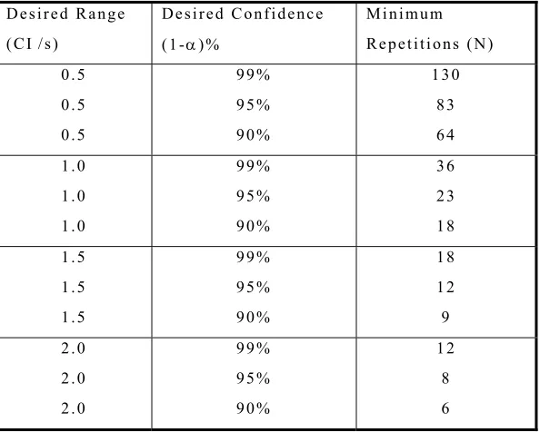
The required minimum number of model repetitions is computed by the following statistical formula (13):
CI (1-α)% = 2*t (1-α/2), N-1 *( s /(√N))
Where,
CI (1-α)% = the (1-alpha)% confidence interval for the true mean, where “alpha” equals the probability of the true mean not lying within the confidence interval.
t (1-α/2), N-1 = the Student’s “t” statistic for the probability of two-sided error summing to “alpha” with (N-1) degrees of freedom, where “N” equals the number of repetitions.
s = the standard deviation of the model results.
32
Table 3.1: Minimum Repetitions to Obtain Desired Confidence Interval
Desired Range
( C I / s )
D e s i r e d C o n f i d e n c e
( 1 -α)%
Mi ni mum
Re pet iti ons (N)
0 . 5
0 . 5
0 . 5
9 9 %
9 5 %
9 0 %
1 3 0
8 3
6 4
1 . 0
1 . 0
1 . 0
9 9 %
9 5 %
9 0 %
3 6
2 3
1 8
1 . 5
1 . 5
1 . 5
9 9 %
9 5 %
9 0 %
1 8
1 2
9
2 . 0
2 . 0
2 . 0
9 9 %
9 5 %
9 0 %
1 2
8
6
* Desired Range = Desired confidence interval (CI) divided by standard deviation (s). Source: (CALTRANS / Dowling et. al., 2002)(13)
The confidence interval is the range of values within which the true mean value
may lie. For a desired range of confidence interval (CI/s) of 1.0, and a confidence level of
95%, the minimum number of repetitions required will be 23. For a narrower range of the
confidence interval such as 0.5, at 95% confidence level, the minimum number of
repetitions required will be 83. The number of model run repetitions (each using different
random number seed) is obtained by using an iterative process. An estimate of the
variance of model MOE (such as mean flow rate, mean delay) is required to estimate the
number of model repetitions, either from past experience or by running a few model runs.
After a few model runs, an initial estimate of standard deviation is obtained and the
number of repetitions is determined using the above statistical formula for the desired
confidence interval. This initial estimate of the standard deviation is revisited or revised
Model Based Sensitivity Test:
A check on the number of model repetitions determined from the use of statistical
formula is performed by looking at the variability in the model output and the number of
outlier runs. The outlier runs represent network gridlocks with far higher values of system
queue delay and lower total throughputs. The check on the number of model repetitions is
performed by running sets of 25, 50, or 100 model runs and examining the range of
distribution of the model outputs. In the case of the test bed the model based sensitivity
test was performed for the non-calibrated model. Figure 3.4 presents the distributions of
system queue times for the three sets of model repetitions for 4-6 PM period. The outlier
runs were those having system queue time values greater than 4 standard deviations from
the mean. There were seven such outlier runs in the case of 100 runs, four in the case of
50 runs and only two in the case of 25 runs.
Figure 3.5 presents the number of outlier runs versus the number of model
repetitions. Based on 100 model repetitions, the probability of occurrence of an outlier
run is 7%. The proportion of outlier runs in all three sets of runs ranges from 7% to 8%.
This shows that there is no appreciable difference in the chance of occurrence of the
34 Comparison of System Queue Time* (p622a) 4-6 PM
For 100 Runs: Mean = 545 veh-hrs, S.D=168 For 50 Runs: Mean = 531veh-hrs, S.D = 161 For 25 Runs: Mean = 531 veh-hrs, S.D = 131
0 5 10 15 20 25 30 35
400 480 560 640 720 800 880 960 1040 1120 1200 Queue Time (veh-hrs)
* 2, 3, & 7 Outlier Runs Removed From Analysis of 25, 50, & 100 runs respectively
Fr
eq
ue
ncy 100 Runs
50 Runs 25 Runs
Figure 3.4: Comparison of system Queue Time for 25, 50, and 100 Model Repetitions for the Non-Calibrated Model
Number of Outlier Runs versus number of Model Repetitions
Uncalibrated Model (Case: p0622a); 4-6 PM
0 1 2 3 4 5 6 7 8
Number of Model Repetitions
Number of O
utlier Runs 25 Runs
50 Runs 100 Runs
Table 3.2 presents the mean, median, and standard deviation of the system queue
delay for the three sets of model runs. Given the fact that outlier values were removed
from the analysis, a comparison of the standard deviation values presented in the table
shows highest variance in the case of 100 runs followed closely by set of 50 runs. The
lowest variance in the system MOE was generated by set of 25 runs.
Table 3.2: Comparison of Total Queue Time (veh-hrs) from Different Number of Run Repetitions for Non-Calibrated Model (4-6 PM)
Number of Model Run Repetitions
25 50 100
Mean* 548 535 545
Median* 492 480 476
Std. Deviation* 152 161 168
* Excluding values of outlier runs
Table 3.2 also shows that the median values of system queue time for 50 and 100
model runs are fairly close to each other at 480 and 476 veh-hrs respectively. The median
values were less affected by the outlier runs as compared to the arithmetic mean values
which are greatly affected by these extreme data points. The benefits of achieving higher
accuracy by using higher number of runs should be weighed against the extra time and
effort required in running the model and the analysis. In practice there are constraints on
these resources and therefore given the marginal increase in the model reliability afforded
by higher number of runs such as 100 runs over 50 runs in the case of the test network,
usually the later should be sufficient from a practical stand point.
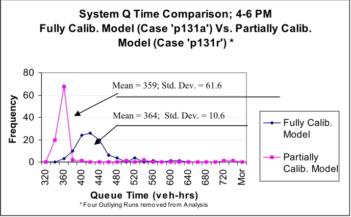
For the purpose of comparison, a partially calibrated model for the test network
was also tested for variance in the model MOE. The partially calibrated model showed
fewer outlier runs than the non-calibrated model because of the fact that the driver
behavior parameters related to spillback probability and gap acceptance were calibrated
to replicate the real world conditions in the case of the former. A graph similar to the one