Integrated link level and circuit level simulation of mobile communication systems

Integrated Link Level

and

Circuit Level Simulation

of

Mobile Communication Systems

J

eyhan Karaoguz

Center for Communication and Signal Processing

Department of Electrical and Computer Engineering

North Carolina State University

Raleigh, North Carolina

.

November 1989

KARAOGUZ, JEYHAN. Integrated Link level and Circuit Level Simulation of

Mobile Communication Systems. (Under the direction of Michael B. Steer and

Sasan H. Ardalan)

This thesis discusses the development of a simulation environment for the

anal-ysis and design of RF communication systems from the link level down to the

nonlinear RF circuit level. The integrated simulation environment supports block

diagram representations, multirate sampling, and an interactive graphical user

in-terface. It enables the incorporation of sophisticated user models of individual

blocks, in a mixed time-domain and frequency-domain environment.

The simulation of a multi-channel mobile communication system is presented.

The integrated link level and circuit level simulation environment is used to

de-termine the large-signal nonlinear distortion effects such as harmonic distortion,

intermodulation distortion and spurious noise which are due to the RF receiver

front-end. Also presented are the results of large-signal distortion effects on the

adjacent channel interference and signal to noise ratio.

Finally, the simulation results are compared to measured receiver front-end

Table of Contents

1 Introduction

1.1

1.2

Motivation For This St udy

Thesis Overview .

...

...

1

1

2

2 Review of Computer-aided Techniques for Communication

System Analysis and Design ₅

2.1 Discussion of Terms: Modeling, Simulation, and Simulation Model 5

2.1.1 The Aid of Simulation Modeling in Communication Systems

Analysis and Design

2.2 Review of Previous Work .

Discussion and Conclusion . . . . 2.3

2.2.1

2.2.2

2.2.3

Computer-aided Analysis and Design Techniques.

Simulation Based Methods . . . .

Communication System Modeling

6 7 8

10

3 Integrated Simulation Environment Design

3.1 Introduction .

21

21

3.2 General Structure and Functions of the Integrated Simulation

Environment . . . 22

3.2.1

3.2.2

Link level Simulation: CAPSIM . .

Circuit Level Simulation: FREDA

23

3.3 Summary · . · · · ·

4 The Simulation System: Mobile Communications

33

34

4.1

4.2

4.3

Introduction. . . · · · ·

Technical Problems in Mobile Communication Systems ·

4.2.1 Link level Impairments . . . .

4.2.2 Circuit Level Impairments.

Description of Mobile Communication System.

34 35 35 36

38

4.3.2

Description of Link Level .

Description of Circuit Level

38

41

5 Methodology and Implementation of Mobile Communication

System Simulation

5.1 Introduction . . .

43

43

5.2

5.3

Simulation Procedure

Functional Description of the Simulation Example

43

46

5.3.1

5.3.2

5.3.3

Transmitter Galaxies. . . .

Transmission Medium Galaxy.

Receiver Galaxy .

46

48

50

6 Simulation Results and Discussion ₅₃

6.4 Noise Distortion .

6.5 Adjacent Channel Interference

6.2

6.3

6.6

Harmonic Distortion . . . .

Intermodulation Distortion

IF Spectrum for 29 Incommensurable Input Frequencies

54

58

65

72

80

RF Power vs. IF Power Measurements

7 90 kHz Experiment

7.1 Introduction . . .

7.2

7.3

7.4

7.5

Experimental Setup

Noise Measurements . . . ·

Conclusion and Discussion ·

...

82

82

89

Suggestions for Further Study

8.1

8.2

8.3

Summary

. .

.

. . .

. .

.

.

.

.

.

.

.

.

.

. .

.

.

.

.

.

.

.

.

.

.

.

.

.

...

96

A Detailed Software Structure of Integrated Simulation Environment 106

A.I

A.2

Introduction . . .

CAPSIM Software

...

...

106

A.4 Interface.

109

B User's Guide

.

.

...

113

B.1

113

B.2 CAPSIM Environment .

...

113

B.3 FREDA Topology

120

B.4 Terminal Session

...

124

Introduction

1.1

Motivation For This Study

Digital communications and computers are having a tremendous impact on the

world today. The number of technologies available for providing a given service is

growing daily, covering transmission media (microwave and coaxial cable

transmis-sion, optical communication via fibers and space satellite transmission), devices

(GaAS and silicon devices and VLSI circuits), and software (protocols, system

ad-ministration, diagnostics, and maintenance). The resulting design, analysis, and

optimization of performance can be very demanding and difficult.

Many computer-aidedtechniqueshave been introduced in recent years to assist in the modeling., analysis, design and testing of communication and signal

process-ing systems. Although there have been significant developments in computer-aided

modeling, analysis, and design of communication systems, there are still some

es-sential issues which ·have not been addressed strongly or not at all. One of the

important issues is the amalgamation

[1]

affect the performance of others, and sometimes it is extremely difficult to isolate

a part of the system from the others except in some oversimplified cases.

The problem of estimating the performance of the circuit level in the presence

of all link level sources of impairments such as inter- and co-channel interferences,

up- and down-link noise

[2]

environment. The objective of this study is the development of such an integrated

simulation environment concept. In particular, the study presents a multi-channel

mobile communication system simulation to verify the operation of the proposed

integrated simulation environment.

The following section provides an overview of the organization of this thesis.

1.2

Thesis Overview

Chapter 2 presents a thorough literature review of the computer-aided techniques

for communication system analysis and design. Different level simulation tools are

described and their performances are evaluated. Another purpose of this review

section is to familiarize the reader with the large amount of terminology used in

this area, and place the proposed simulation environment into the proper category.

Chapter 3 is devoted to the development of the integrated simulation

environ-ment. The different level simulators, CAPSIM and FREDA, which were used to

concepts and procedure in interfacing FREDA into CAPSIM are given. The

fea-tures of the integrated simulation tool are summarized briefly at the end of that

chapter.

Chapter 4 explains the reasons for choosing mobile communication systems as

the simulation example. The technical problems which make the mobile

communi-cation systems challenging for design and analysis purposes are presented. Finally,

the chapter ends with the detailed description of the general mobile

communica-tion system at the link and circuit level.

Chapter 5 focuses on the implementation of the simulation example. After

the introduction of the simulation procedure, the functional descriptions of the

individual blocks which build up the system are given. The incorporation of the

link level and circuit level impairments into the operation of functional blocks is

presented.

Chapter 6 presents the results of the simulation example implemented in

Chap-ter 5. The results include the harmonic and spurious response of the nonlinear RF

mixer circuit, intermodulation distortion, adjacent channel interference and noise

distortion. Along with the .results, the large signal nonlinear distortion effects of

the link level impairments on the RF circuit level are discussed.

Chapter 7 presents the 90 kHz receiver front-end experiments. First the

exper-imental setup is introduced. Then the results for conversion loss (RF powerVB. IF

Chapter 8 contains the summary, conclusion and suggestions for future study.

Appendix A presents the detailed software structure of the integrated

simula-tion environment. The user's guide for the simulasimula-tion tool is given in Appendix

B. The C-programming codes for the stars (building blocks) are provided in

Chapter

2

Review of Computer-aided Techniques for

Communication System Analysis and Design

2.1

Discussion of Terms: Modeling, Simulation, and

Simulation Model

Before starting the review section, we would like to clarify and discuss the meanings

of the terms modeling, simulation, and simulation model since these terms are

frequently used throughout the thesis.

Modeling and simulation have been practiced ever since there were difficult

problems to solve and complezobjects to describe. Modeling can be simply defined as creating any abstract representation of something or some activity short of the

real thing or the thing-to-be. For example, a model can be a mental picture or

concept, a sketch, a description, a set of plans, a set of mathematical equations,

a computer program, a pattern, etc. It is a means by which something which

is modeled can be explained, expressed, presented, or studied. Simulation, as

defined by Webster's, is "the act or process of giving the appearance or effect of".

Thus, in general, the two terms modeling and simulation are quite synonymous.

sense one may say that simulation is a process by which model( s) of something or

an activity is exercised or stimulated to produce the effects (on certain objects)

similar to or relatable to that of the real object or activity. It is also in this rather

limited sense that the term simulation model is used - a model specifically built

for simulation.

2.1.1

The Aid of Simulation Modeling in Communication

Systems Analysis and Design

The complexity of communication and signal processing systems has grown

con-siderably during the past years. As the growth in the subtleness of the system

has increased, the analysis and design have become demanding and difficult. Also

the rapid emergence of the new technologies has made many existing products

obsolete and therefore has created a competitive market for new products. This

aspect of technology requires engineers to design new products in a timely, cost

effective, and error free manner. These demands can be met only through the use

of powerful computer-aided analysis and design (CAAD) tools [3].

A large body of computer-aided techniques have been developed during recent

years to assist in the process of modeling, analyzing, designing and testing

com-munication and signal processing systems. Each of them has its own approach

both analytical and simulation, to guide the analysis and design throughout the

life cycle of a system [4]. Performance evaluations and tradeoff analysis are the

central issues in the design of communication networks, links and circuits.

Dig-ital simulation provides a useful and effective means to direct analytical

evalu-ation of communicevalu-ation system performance. Indeed there are many situevalu-ations

where explicit performance evaluation defies analysis and meaningful results can

be obtained. only through either actual prototype hardware evaluation or digital

computer simulations [4].

The interactive nature of different levels - network, link, circuit and signal

processing level - make the design and analysis of communication systems a

chal-lenging task for engineers. Therefore in the communications industry, designers

are looking into means to analyze the whole communication system interactively.

The top-down analysis of communication systems is essential because the

perfor-mance and response of the circuit level strongly depend on the network or link

level, and vice versa. Except for some idealized and often oversimplified cases, it is

extremely difficult and time consuming to find analytical or closed form solutions

to this aspect of the system.

2.2

Review of Previous Work

In this section, computer-aided modeling, analysis, design and simulation tools

performances of these CAAD tools are evaluated.

2.2.1

Computer-aided Analysis and Design Techniques

Computer-aided techniques for system analysis and design can be divided into two

categories

[5] :

• Formula Based Approach - In this approach, computer is used to solve sets of equations in finding closed-form solutions .

• Simulation Based Approach - In this case, computer simulates voltage and current waveforms or signals that flow through the system.

The basic distinction between the two is that formula-based models are

im-plemented as mathematical expressions that are usually oriented towards some

measures of merit (e.g., performance), whereas simulation models are designed to

emulate functions and are oriented towards stimulus and response (e.g.,

input-output signals). Both of these approaches have unique sets of advantages and

disadvantages. These are further discussed as follows.

The formula-based model [6] requires only a suitable mathematical model to

represent, for instance, the performance of a receiver subsystem such as the

demod-ulator/detector. The advantages [5] of -the formula-based or so called analytical

i)

ii) computer implementationis usually quite straight forward and efficient

with-out requiring a great amount of computer storage.

iii) computation time is generally short and, hence easily accommodated.

The major disadvantages of the analytical modeling approach are the lack of

flex-ibility in representing different implementation methods, and the limited depth or

accuracy of the system which depends on the adequacy of the analytical

descrip-tion. Also, the formula-based mathematical techniques require that the system

models be simple, thus serving to broadly explore the design space.

II: .he simulation modeling approach, the same demodulator/detector as

men-tioned above would have to be numerically represented and implemented. In effect,

the numerical implementation would be closely equivalent to actual hardware

im-plementation. Given the required numerical model, a simulated numerical input

signal(s) could be applied to the simulated demodulator/detector. The

advan-tage of this approach is that the simulated demodulator/detector could be used

again and again to generate and evaluate the responses to different input signal

characteristics. Additionally, the simulation approach does not require a priori

information about the received signal vector. With simulation-based techniques,

systems can be modeled to any arbitrary level of detail, and hence the design

space can be explored more finely. The major disadvantage, however, is that a

ongo-disadvantages of the simulation modeling approach.

Based on the above observations, the best approach would be to structure

the simulation software primarily to support the simulation modeling approach

with enough flexibility to support the incorporation of analytical models. As

an example,

CLASS [7,8]

formula-based analysis for evaluating the performance of satellite communication

systems. Although, these two different techniques are complementary in that many

simulation based techniques now incorporate formula based results to reduce the

computational burden, the simulation based approach has become the primary

tool for modeling and analyzing complex communication systems, and therefore

is the subject of this thesis.

2.2.2

Simulat'ion Based Methods

The simulation based methods have gone through different phases throughout their

existence. The aspects that have changed are their approaches to communication system simulation, the languages of simulation packages, and the host computers

used.

First, an examination of the different approaches to communication system

simulation shows that in the early days, users wrote individual programs to

design [3]. These programs were typically executed on a main-frame computer in a

batch mode, and the simulation output consisted primarily of numbers and tables.

A considerable portion of the engineer's time was spent in writing and debugging

the programs rather than on modeling and analysis [3]. Block-oriented approaches

to modeling and simulation such as MIDAS, SCADS, and CSMP [9,10,11] were

developed in the early 1960's for digital simulation of analog systems. This

ap-proach eliminates the need for the user to write simulation code. Block-oriented

simulations draw their motivation from the analog block diagram as a simple and

convenient way of describing continuous systems [12]. Advances in discrete-time

systems and signal processing have led to new approaches for digital

communi-cation system simulation. Software packages for simulations based upon

trans-form domain techniques (FFT for frequency domain and biliniar-Z transtrans-form for

time domain techniques] began to emerge in the late 1960's and early 1970's.

S}TSTID [13,14], CMSP, CHAMP [15,16], LINK [17] and others [18,19] were

developed in this time frame. The state of the art block-oriented simulators, such

as BLOSIM IC AP51M [20,21] and BOSS [22], provide an interactive framework

for simulation-based analysis and design of communication systems with

capabili-ties to 1) develop simulation models in a hierarchical fashion using graphical block

diagram representations,

2)

review the results of simulations, and 4). perform design iterations.

level languages such as FORTRAN etc. Unfortunately, those higher level languages

lack the opportunity

[4]

of the block-oriented approach. Therefore today's software simulation packages

tend to have a pre-processor to a lower level language. This approach lends itself

to portability and frees the user from having to know the details of the underlying

operating system and the hardware configuration of the simulation facility. The

pre-processor STARGAZE

[23]

Finally, the host computer environment has changed as the computer

hard-ware advanced. In the early days, circuit and control analysis softhard-ware tools (e.g.,

ECAP, SCEPTRE, AIIMIC

[14])

cer-tain systems in the time domain. However, both methods had serious drawbacks,

including excessive computer run time and step-up complexity. This was

particu-larly true when addressing complicated problems involving performance analysis

measurements, such as noise power ratio, and when simulating systems with low

bit error rates. In the past ten years, computer hardware and software have

un-dergone significant changes. Powerful workstations such as the

SUN, APOLLO,

VAX

offer friendly computing environments with highly visual and graphical user

inter-faces. Considerable effort is currently directed towards developing intelligent and

workstations as well as PC technologies

[12].

that take full advantage of the hardware/software environments offered by

work-stations are CAPSIM

[21]

[22].

for simulation-based analysis and design of communication systems with the

ca-pability for developing simulation models in a hierarchical fashion using graphical

block diagram representations. For many applications, PC's are preferred because

they not only provide sufficient power for simulation- based analysis and design of

communication systems, but they are also low cost and provide complete control

over the simulation environment since they are rarely a shared resource. Some

examples of PC-based software packages are the PC version of lCS

[24]

as ll'eS, and

uooeu

[25].

Numerous simulation packages have been introduced, serving different levels of

the communication systems. Desirable features of a simulation package are defined

as follows

[12] :

• Modular Structure - In order to provide maximum flexibility, simulation

packages used to aid communication system analysis and design should have

a modular structure.

• Simulation Programming Language - Fortran, Pascal, or C do not allow

input via block diagrams. Therefore a pre-processor simulation language is

needed, or object oriented languages such as C++ and objective C may be

age should permit the design engineer to connect the functional blocks in

any desired topological interconnection, providing maximum flexibility.

• Model Library - The usefulness of a simulation package depends heavily on the availability of a model library containing many models of various

functional blocks that make up transmission systems and networks.

• Time and Event Driven Simulation - For maximum flexibility, provisions should be made for both time driven and event driven modes of processing

so that event driven blocks can be used interchangeable with time driven

blocks.

• User Interface - Finally, the whole simulation package should be made user friendly.

2.2.3

Cornmunication System Modeling

For the simulation of communication systems, it is convenient to model the system

using three lavels as in Fig. 2.2.1.

The network level [26] is made up of switches (nodes), mtiltiplexers, and

con-centrators connected by means of transmission systems. The transmission link is

composed of communication media (transmission channel and noise), modulators,

NETWORK LEVEL

LINK LEVEL

CIRCUIT

AND

SIG. PROC. LEVEL

Figure 2.2.1: Hierarchy of CAAD Tools

mixers and other circuits.

Network Level CAAD Tools

Network level CAAD tools are based on computer aided analytic techniques,

sim-ulation, or emulation. In the first two techniques, which are sometimes combined,

the network performance is evaluated using abstracted functional models [27]. In

the third technique, the user specifies the network protocols in great detail [28],

often supplying an actual program implementing the protocol, and these protocols

are then simulated. Tools in this category are called emulators or iestbeds [3].

proto-techniques or tables are used to specify the nodes and interconnecting links. The

modeling of the protocols involves specifying the data structures and the rules that

govern the flow and modifications to the data structures. Three broad approaches

are currently being used for this. The first approach consists of graph based

mod-els such as finite state machines, and petri-nets. These modeling approaches are

typically used for protocol specification and validation. The second modeling

ap-proach uses an extended queuing paradigm. This model is suitable for analytic

solution of network performance obtained via queuing theory. In the third class

of models, the protocol functions are specified as a collection of interacting

proce-dures. This approach is based on the fact that network protocols are algorithmic

in nature, and a signal flow type block diagram can express the algorithmic nature

of protocol functions clearly.

In network level CAAD tools, event driven simulation is used, since network

functions process packages of data such as arrival and departure of messages,

occurrences of transmission errors, etc

[12].

for communication networks are available. BONeS [29] is an example in this

category.

Link Level CAAD Tools

Whereas network level CAAD tools use event driven simulations, link level CAAD

a signal flow block diagram form where each block performs a functional operation

like modulation, coding, filtering, etc. The simulation approach consists of

gener-ating sampled versions of all the input signals, processing them through functional

blocks in the model, generating sampled values of the output signals and analyzing

them to extract performance measures. At the link level, the end-to-end

perfor-mance [26] is measured in terms of waveform distortions, output signal-to-noise

ratios, and error probabilities as a function of link level parameters such as filter

bandwidths, power levels of input signals and noise, operating point of amplifiers

and nonlinear circuits, and so forth.

Systems and signals are represented in the discrete time domain using sampling,

and bandpass signals are usually represented by their complex lowpass equivalents

[30]. Monte-Carlo techniques [31,32,33] are used to handle random variations in

signals and systems and simulation is run long enough to accumulate enough

sam-ples to obtain statistically valid estimators of performance measures. However the

computational burden of Monte Carlo simulations is considerable. For example,

if Monte Carlo simulations are used to estimate the unknown error probability in

a digital communication link, several million symbols will have to be processed

during the simulation in order to obtain statistically accurate estimators of low

probability (on the order of 10-6

) [26]. The processing time for this may approach

the order of several hours to days. A number of techniques are currently being

Circuit and Signal Processing Level CAAD Tools

One of the primary areas in which engineers are most involved is circuits. Until

now, many software packages have been introduced such as SPICE [35,36] and

FREDA [37]. The basic difference between link level and circuit level simulation

packages is that link level CAAD tools are generally simulation environments for

time driven waveform simulations whereas circuit level CAAD tools are based on

solving a set of linear or nonlinear differential equations resulting from application

of Kirchoff's voltage law and Kirchoff's current law using constitutive relations

(i.e., the element characteristics). The methods for circuit level simulation may

be characterized into three groups by the way in which the circuit elements are

treated: Time Domain Methods, Hybrid Methods, and Frequency Domain Method»

[37].

In time domain methods both linear and nonlinear elements are analyzed in

the time domain. The numerical integration of the circuit parameters is used. The

time domain methods are useful if the transient response is desired but inefficient

when the circuit has widely varying time constants or the signal is widely separated

in frequency. A widely used time domain circuit simulator is

SPICE

hybrid methods use time domain analysis for the nonlinear elements, and frequency

domain analysis for the linear elements [38,39]. These methods directly calculate

the entire circuit is analyzed in the frequency domain without transformations

between the time and frequency domains. FREDA is an example of a frequency

domain circuit simulator [37].

The availability of low cost/high speed signal processing hardware has allowed

the increasing use of digital signal processing in many areas. With the drive

towards all digital communication networks, significant portions of the

communi-cation systems use complex signal processing techniques, and an increasing need

exists for CAAD tools which can aid in the design of these systems. Many of the

currently available signal processing simulation tools perform analysis and design

of only specific DSP algorithms and functions, such as FIRand IIR filtering. One

of the few examples in this category is SPW(Signal Processing Worksystem)

[3].

2.3

Discussion and Conclusion

In this chapter, computer-aided design, analysis, and simulation tools for

commu-nication networks, links and circuits were surveyed.

There is no doubt that the complexity of modern communication systems

whether they are at the link, network or circuit level, require an extensive use

of

CAAD

design of communication systems, it imposes some problems to be addressed as

well.

coded communication systems operating at low error rates may take several

hours of cpu time .

• The development of an expert ~Y3temfor simulation based de3ign - At the present time simulation is primarily used as an analysis tool, with the

engi-neer making heuristic choices for design iterations on a trial and error basis

which is time consuming and inefficient.

• The integration ofsimulation tools - There is a lack of integration between simulation tools within and between the various levels of the hierarchy shown

in Fig. 2.2.1. There is a considerable amount of "hand transfer" of data

be-tween various CAAD tools which is the cause of numerous design errors and

delays. An integrated environment for CAAD tools is essential for improving

productivity and minimizing costly errors.

In this thesis, we are going to deal with the latter problem and present a

simulation environment which integrates different level CAAD tools, namely, the

link and circuit level. The practical use of this integrated simulation environment

Chapter

3

Integrated Simulation Environment Design

3.1

Introduction

Conceptually, the need for amalgamating the link level simulation with that of

the nonlinear RF circuit level led to the design of an integrated communication

system simulation environment. The main goal for this integrated environment

is the development of an hierarchical approach to simulation which permits the

use of multiple tools within the environment and a hierarchy within each level

of the system as well. A simulation tool at an intermediate level accepts data

from the lower level modules and provides data to the models used in the next

higher level. By loosely integrating the simulation tools at successive levels in

the hierarchy through a flexible interface, an integrated environment has been

achieved for the simulation and design of communication and signal processing

systems. Also considered were the provisions for merging different circuit level

Simulation Errvir-onrnent

The integrated simulation environment is a mixed time domain and frequency

domain simulator. Mostly frequency domain processing has been employed in the

simulation environment. Frequency domain processing is more advantageous for

linear functional blocks such as filters. It permits the use of measured values of

filter characteristics such as amplitude and phase response [4].

The sampling rate is an important issue in communication system simulation.

Especially for RF communication systems, the baseband signal can be many

or-ders of magnitude lower than the frequency of the RF signal. This has led to the

complex envelope representation of signals and baseband equivalents of

subsys-tems to reduce the sampling rate [30,40,41]. However, when we are dealing with

nonlinear systems, this technique is inappropriate since nonlinear characteristics

involved in the frequency translation from RF to baseband are not captured. By

the same token, any functional operation such as filtering or passing the signal

through a nonlinear transmission medium has different effects on the baseband

signal than it would have for the RF signal. This characteristic of the system

precludes using the complex envelope and baseband equivalent representations of

the bandpass signals. In time domain analysis, a remedy seems to be to increase

the sampling rate, but this is very inefficient. For the proposed integrated

for bandpass signal processing. What is meant by representing the bandpass

sig-nals in frequency domain is that only the RF frequency part of the spectrum is

retained since the spectrum elsewhere is redundant. Accordingly, all functional

blocks process the RF signal spectrum at this RF carrier related frequency.

The designed CAAD tool can be divided into two parts, i.e., CAPSIM (link

level simulator) and FREDA (nonlinear RF circuit level simulator). CAPSIM and

FREDA have different approaches to simulation since they are dealing with

differ-ent levels of the system. The integrated simulation environmdiffer-ent is the appropriate

interface of FREDA to CAPSIM. Before proceeding with the interface procedures,

next two sections describe CAPSIM and FREDA.

3.2.1

Link level Simulation

CAPSIM

CAPSIM

[21]

analysis of communication systems. The integrated environment includes the

ca-pability to design models, subsystems, and systems in a hierarchical fashion using

block diagrams. CAPSIM is a refinement and extension of the time-driven block

diagram simulator BLOSIM [20]. The BLOSIM simulator was chosen because of

its hierarchical block orientation and many other desirable features; however it has

the drawback of being text oriented. CAPSIM was designed to allow BLOSIM to

be used much more easily and efficiently.

op-to specify the design in a hierarchical manner using block diagrams which are

fa-miliar to system designers. CAPSIM provides a complete interactive environment

for communication system design and engineering. The integrated environment

includes the capability of defining blocks and models in a hierarchical fashion,

configuring and executing a simulation, reviewing the results of simulation, and

performing design iterations. Each of these capabilities is controlled through a

user interface using interactive graphical techniques.

CAPSIM is essentially a time-driven simulator and each block is polled at each

sampling instance. Multirate sampling techniques enable the simulation of many

systems whose blocks have different bandwidths.

CAPSIM Approach

Philosophically, CAPSIM is closest in approach to writing a special-purpose

sim-ulation program, and offers similar advantages of efficiency and generality. At the

same time it overcomes the deficiencies of many special-purpose simulation efforts

by providing a structured environment for programming simulations. This

struc-tured environment encourages the programmer to use highly strucstruc-tured

program-ming techniques, but without requiring any prior familiarity with these techniques.

This means that CAPSIM frees the user from having to contend with simulation

house-keeping duties. Instead, the u~er may concentrate on the functions of the

divi-dends. First it encourages the writing of simulation code for small pieces of the

system being simulated, and this code is written to a single carefully defined

in-terface. As a result libraries of routines, re-usable in future simulations, can be

developed. Second, multiprogrammer simulation efforts become relatively painless

since routines written by different programmers readily interface to one another

[20].

The terminology that is used in CAPSIM in describing the different types of

blocks is, as in BLOSIM, modeled after cosmology: A block which is elementary

or atomic in the sense that it is implemented directly by a user-provided routine is

called a star. A block which is defined as a connection of other blocks, on the other

hand, is called a gala:vy. Finally, a special galaxy is defined which encompasses

the entire systems, and which therefore has no inputs or outputs. Such a galaxy

is known as the universe. By definition, unlike all other blocks, the universe

can only have a single instance. The cosmology of blocks differs from ordinary

cosmology in that a galaxy need not contain exclusively stars, but rather can

contain other galaxies. There is no limit on the nesting of galaxies

[20].

The Pre-processor

A star consists of code written in pseudo C-code. The statements themselves are

legal C operations, but the star is not an executable C-program. Before the star

can be used, it must be passed through the stargaze pre-processor which produces

pre-pseudo C-code into an ordinary C-program. The user can easily define new stars

to perform almost any function of interest. To facilitate the introduction of a new

star into CAPSIM, a pre-processor called pre-capsim has been designed. This

pre-processor creates the object code for the star, and after leaving a COPJTof this code in an individual user library, links this code with the remainder of the object

modules related to CAPSIM. The result is the creation of a customized version of

CAPSIM which contains only the stars needed by that specific user. This allows

different users to have their own customized version of CAPSIM, containing the

stars necessary for their individual simulations.

Simulation Configuration

CAPSIM supports a hierarchical definition of blocks. That is, it is simple to define

new blocks which are made up of specified interconnections of other blocks. In

subsequent simulations, these higher level blocks are indistinguishable from blocks

implemented directly by a user program. In addition, multiple instances of blocks

are supported. That is, the same block can appear as many times as desired in

a given simulation (usually its functionality is specified by setting different values

for its parameters). This is particularly convenient for simulation systems which

have a replication of similar or identical functions (for example a systolic array of

or a system with multiple filters). CA,PSIM also makes many consistency checks

user programming errors. The scheduling of the order of execution of the blocks

in the universe is done without regard to whether the blocks are stars orgalaxies.

All the blocks are examined to find any which have no inputs. These blocks are

scheduled to execute in arbitrary order. At step k, all the blocks which have not

been scheduled in steps 1throughk-l are examined to find any which have inputs connected exclusively to blocks which have been scheduled in steps 1 through k-l.

Blocks satisfying these criteria are scheduled next in arbitrary order. These steps

are repeated until all blocks within a universe have been scheduled.

A user defined topology is constructed by selecting blocks from the menu

and placing them on the work space. As each block is selected, the user will

be prompted for parameters if needed.

The Post Processor

The results of simulation are displayed using signal plotting and processing

tech-niques. The outputs of the simulation may be sent to a text file for manipulation

by another program or can be used as inputs to subsequent CAPSIM simulation.

The post processor uses the same interactive graphic interface to allow the user

to select signals from the block diagram for display and manipulate the plotting

FREDA is a nonlinear RF circuit simulator described in [37] and [42]. Although

the methods for analyzing nonlinear RF circuits are varied, they are all based

on solving a set of nonlinear differential equations resulting from application of

Kirchhoff's voltage law and Kirchhoff's current law using the constitutive relations

(i.e., the element characteristics). The methods fall into three groups according to

the way in which the nonlinear elements are treated: time domain methods,

hy-brid (harmonic balance) methods, and frequency domain methods. Time domain

methods analyze the nonlinear circuit by solving the nonlinear differential

equa-tions governing the circuit in the time domain using a method related to numerical

integration

[43].

circuit analysis. Microwave and RF circuits typically have widely separated time

constants resulting in a set of stiff state equations. The consequence is that a small

time step must be chosen and simulation must proceed for a large number of time

steps leading to excessive computation time. Furthermore, it may be difficult to

identify the steady-state solution when closely spaced frequencies are present.

The hybrid methods avoid the numerical integration of the state equations as

required in the time domain. These methods directly calculate the steady-state

response of the nonlinear circuit, and are generally referred to as harmonic balance

methods. The modern version of the harmonic balance method was presented in

partitioning the network into smaller sub-networks that are composed of either

linear circuit elements or nonlinear elements. The linear sub-networks are solved in

the frequency domain while nonlinear sub-networks are solved in the time domain.

Several variations of the harmonic balance method in [38] have been proposed to

handle nonharmonically related signals. The modified harmonic balance methods

are presented in [39,44,45,46,47].

The frequency domain methods avoid explicit time domain calculations. This

is accomplished through the use expansion of the input-output characteristics of

the nonlinear elements in a set of basis functions. There are three types of basis

function expansions: Volterra series, algebraic functional expansion, and power

series. Volterra series techniques can only be used to analyze weakly nonlinear

systems [37]. The algebraic functional expansion method is related to Volterra

series, but the analysis procedure is quite different

[48].

spectral balance analysis, power series based techniques are proving to be the most

general methods for the analysis of nonlinear circuits with multi-frequency large

signal excitations and are easily integrated into existing computer-aided design

tools [37].

FREDA implements the harmonic balance and frequency 'domain methods of

nonlinear RF circuit analysis [37,42]. Both methods implement the spectral

bal-ance procedure as follows. A nonlinear analog circuit is partitioned into linear and

Of

t t·

-+---

---..

"

-.l

LINEAR

I I

NONLINEAR

SUBCIRCUIT v ELEMENT

T

--

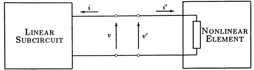
Figure 3.2.1: Partitioning of a microwave circuit into linear and nonlinear subcir-cuits for harmonic balance analysis

In this example the frequency domain form of the voltage v

==

i (as a set of phasors) into the linear subcircuit is calculated using standard linear

circuit techniques [43]. Then the current _{i '} (again as a set of phasors) flowing

into the nonlinear circuit is calculated using the almost periodic Fourier transform

technique [46,47], the multidimensional fast Fourier transform technique (NFFT)

[49], or the arithmetic operator method (AOM) [37]. (Of these the NFFT method

is preferred for the simplicity in nonlinear device modeling and the AOM technique

for speed and memory usage when there are two or more incommensurable signals.)

Whichever method i~ used in determining the nonlinear curre~ti', a balance of i

and _{i '} is achieved using a Newton iteration scheme to update the estimated voltage

3.2.3

_{Interface of FREDA into CAPSIM}

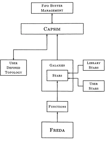
Fig. 3.2.2 illustrates the structure of the integrated simulation environment,

partic-ularly as it relates to the user interface. The user provides three types of routines:

a system topology, star routines (could be system-provided as well), and a

net-list for FREDA. These routines interface to CAPSIM (rather than directly to one

another) which handles FIFO buffer management. The user-supplied "topology

definition" program specifies the names of stars, the routine which implements

each star, and how the stars are interconnected. The topology definition

rou-tine is also able to pass parameters to the stars to specialize their function. The

stars get their input samples from input FIFO's, and put their generated output

samples into output FIFO's.

The functions, in Fig. 3.2.2, are particular routines to be called by a star when

they are needed. Those functions could be an FFT (Fast Fourier Transform),

dig-ital filters, or any other user defined mathematical functions. The convenience

introduced by the functions is that the user can easily implement frequently

needed routines in stars simply by calling functions. FREDA was interfaced into

CAPSIM as one of these functions. More information as to the software details

in the interface procedure is provided in Appendix A. Once the simulation is

exe-cuted according to the user defined topology, FREDA takes over as the nonlinear

RF circuit simulator at the appropriate point in the simulation. By

FIFO BUFFER

MANAGEMENT

CAPSIM

USER LIBRARY

GALAXIES

I

DEFINED

TOPOLOGY ~

STARS

...

L

STARS

FUNCTIONS

FREDA

FREDA is a complete frequency domain simulator, all CAPSIM stars connected

to the FRED A star are forced to process in the frequency domain in order to be

consistent with FREDA through the interface. This transformation is managed

by FFT stars in the CAPSIM system topology.

3.3

Summary

In summary, the incorporation of the link and the nonlinear RF circuit level

simula-tion of the communicasimula-tions systems has resulted in a flexible integrated simulasimula-tion

environment which enables us to see the effects of link level perturbations on the

nonlinear RF circuit level such as the effect of transmission media change on the

received signal at physical level and vice versa. In addition, a great deal of

effi-ciency is achieved in representing the filters and bandpass signals in the frequency

The Simulation System : Mobile

Communications

4.1

Introduction

In choosing an example, we tried to cover a broad range of applications and be

fairly general. The simulation of a mobile communication system was suited to

this objective because of its complexity and the way that the different levels of

the system affect each other. Another motivation in choosing the mobile

commu-nication system as an example is the practical need for an integrated simulation

environment for the design and analysis of mobile communication systems. This

is because, in industry, engineers carry out some field experiments which change

the circuit designs or the modulation schemes accordingly. However, this is a very

costly approach both financially and in terms of the time spent by the engineers to

construct the experiment and take the data. Therefore, an integrated simulation

environment is essential in the design and development of communication circuits

4.2

Technical Problems in Mobile Communication

Systems

The complexity of communication systems has been greatly increased by the

pres-ence of mobile radio technology, although some technical and regulatory issues

still remained unsolved [50]. The allocation of new transmission channels at 900

MHz added many more problems to circuit complexity and analysis as well [51].

Various technical problems make the mobile communication systems difficult for

designers to deal with. These technical problems can be divided into two groups:

link level impairments, and circuit level impairments.

4.2.1

Link Ievel Jmpairmerrts

In the first place, there is a great deal of rnultipath transmission. Because of

reflection from buildings, lamp posts, utility wires, and other obstructions, the

signal may travel from the transmitter to the receiver by many different paths

with different lengths. When one end of the channel is moving, as is usually

the case in mobile communications, the predominant feature of the multipath is

fading. The fading results because, in some relative positions, phases of the signals

arriving from the various paths interfere constructively. Thus as a vehicle moves,

the received signal strength varies erratically and unpredictably over a range of

20 to 30 decibels. Another set of problems that arise in the mobile channel is also

Doppler spreading of approximately

+

leads to other problems such as co-channel and adjacent channel interference. In

a narrow band system the channels can be separated in frequency by 25, 30,

or 50 kHz. Because of vehicle motion, a receiver and a transmitter operating

on adjacent or nearly adjacent channels may be physically close together. The

receiver selectivity must be extremely good to prevent substantial interference

from the strong transmitter signal. Finally, some other problems like intersymbol

interference which results from the arrival of signals at the receiver at different

times are also due to the motion in mobile radio.

4.2.2

Circuit Level Impairments

The problems at the circuit level in mobile communication systems are mostly the

large signal nonlinear distortion effects due to the RF receiver front-end. These

distortions can be localized in the nonlinear RF mixer where the RF signal is

converted down to the IF signal.

As suggested in [52] nonlinear distortion and interference effects in mixers are

those effects which represent departure from the ideal performance when the input

signal in the passband is large. The nonlinear distortion and interference effects

i) gain compression or enhancement - which is a variation of the mixer

con-version gain, or loss, due to the amplitude of the desired input signal.

ii) intermodulation - refers to generation of spurious frequency components at

the sum and difference frequencies of the desired and undesired input signals.

iii) desensitization - modulation of the desired signal by an undesired signal.

iv) detuning - generation of de charge or dc current, due to a large input signal

resulting in a change of the diode bias condition.

In addition to the large signal distortion effects, there is yet another distortion

effect proportional to local oscillator power as well, which had been studied

thor-oughly in

[53].

[53],

then reach a maximum, and finally decrease as local oscillator power increases.

However, the conversion loss is inversely proportional to the local oscillator power,

i.e., the conversion loss decreases as the local oscillator power increases. This fact

suggests a compromise between the nonlinear distortion effects and the conversion

loss.

Another problem related to the circuit level is the inadequate bandpass filtering

at the RF front-end which gives rise to the adjacent channel interference and the

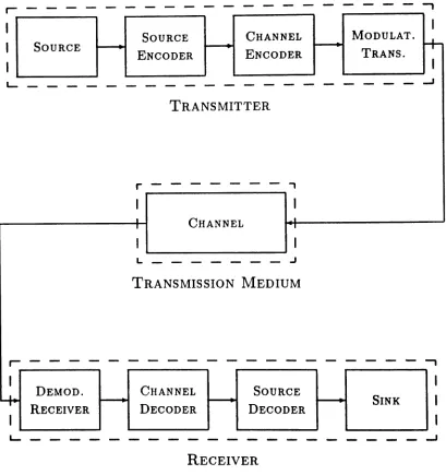
A block diagram is illustrated in Fig. 4.3.1 of a generic communication system

which provides a model for the simulation example. The objective in designing

the simulation example is to include the link and circuit level impairments, i.e.,

to define the individual blocks of the communication system incorporating the

impairments mentioned in Section 4.2. The blocks into which these impairments

are built, are the transmission medium block, i.e., the channel and additive noise,

and the RF front-end block, i.e., the nonlinear RF mixer circuit and bandpass

filter. In the following sections the functional blocks in each level are described.

4.3.1

Description of Link Level

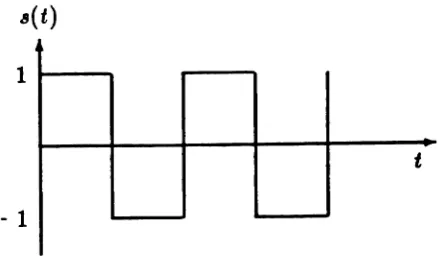
The link level consists of transmitters and the transmission medium. T,,'Po

mitter units are used in order to simulate a multi-channel system. Each

trans-mitter generates a two-tone signal. It is advantageous to use two-tone signals in

the characterization of the channel and in measuring intermodulation distortion

[54]. The purpose of the modulator/translator block in Fig. 4.3.1 is to map the

two-tone signal into a waveform suitable for transmission over the transmission

medium.

The most important block in the link level is the transmission medium block

which is composed of a channel and additive white Gaussian noise. In choosing

I

I

+-I

----..

ENCODER ENCODER TRANS.

I

I

L...

-

-

-

- -

-

- - -

-

- - - -

-

- -

-

-

-

TRANSMITTER

r

-

-

- - - - -

,

I

I

I

CHANNEL I

I I

I

I

L

- -

-

- - -

-

TRANSMISSION MEDIUM

r

-

-

-

- - -

-

- -

-

- -

-

-

-

-

-

-

-

-

I

I

Y.

----..

I

I

I

. - - - .

L... _

---_-.1

RECEIVER

n(t)

FIXED

DELAY

DIRECT PATH

SPECULAR

~MULTIPATH

X

-2:

~ej¢

~---"'fX...--.. DIFFUSE MULTIPATH

To

Differential Delay

Figure 4.3.2: Multipath Path Fading Channel Model

general capability which can support the impairments mentioned in the previous

sections. A physical and practical channel model [40] which satisfies these

re-quirements is a three component fading multipath channel plus additive noise. In

particular, the fading multipath channel is assumed to consist of a single direct

path, a specular multipath component, and a diffuse multipath component as

il-lustrated in Fig. 4.3.2. The quantities

eel

e.

and diffuse multi-path signal energies, respectively, each normalized to the energy

fo are also associated with rnultipath components. The noise component,

n(t)

in Fig. 4.3.2, is an additive white Gaussian noise (AWGN). The noise source is

detailed in the implementation section, Chapter 5. This channel model includes

all link level impairments mentioned in Section 4.2.1.

4.3.2

Description of Circuit Level

At the receiver front-end are the nonlinear RF mixer circuit, bandpass filter, and

the other necessary demodulation blocks.

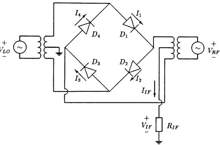
The nonlinear RF mixer circuit is a double-balanced ring diode mixer, as

il-lustrated in Fig. 4.3.3, which is a widely used communication mixer circuit. The

double-balanced ring diode mixer was chosen because of its practical use and its

better performance on harmonic and intermodulation distortion and RF /IF

iso-lation due to its balanced characteristic [55]. The ring diode mixers can also be

used as modulators, phase detectors, and even voltage-controlled attenuators [55].

Therefore, they are very versatile components.

The bandpass filter block is represented in the frequency domain like the other

blocks in the system. It uses measured or independently calculated values for

amplitude and phase response

[4].

the adjacent channel interference because it determines the leakage power from

Chapter

5

Methodology and Implementation of Mobile

Communication System Simulation

5.1

Introduction

This chapter illustrates by way of example the approach that a programmer

us-ing the proposed integrated simulation environment uses to develop a simulation,

particularly the simulation of a multi-channel mobile communication system. The

functional descriptions of blocks (stars) that build up the mobile communication

system are elaborated. The C-programming codes for the stars are provided in

Appendix B.

Next section presents an outline of the simulation procedure as it relates to

the implementation of the simulation example.

5.2

Simulation Procedure

The CAPSIM user can configure a wide variety of digital communication systems

from basic functional blocks, i.e., stars. In the mobile communication system

sim-ulation example, the CAPSIM stars include: signal sources, FFT blocks,

effectively interfaces FREDA into CAPSIM.

The mobile communication system being simulated is illustrated in Fig. 5.2.1

in terms of its implementation in CAPSIM terminology. The detailed descriptions

of the functional blocks follow in Section 4.3. For the purposes of simulation, as

well as actual implementation, the system, i.e., the universe is partitioned into a

number of galaxies. Those galaxies are further subdivided into stars. Each star

is simulated by a user-defined C-program, and the integrated simulation

environ-ment combines these individual simulations into a simulation of entire system.

Before proceeding with the descriptions of the stars, we would like to restate and review the communication between CAPSIM and FREDA, and the

commu-nication within each simulator as well. As mentioned in Chapter 3, there are two

different means to communicate with CAPSIM simulation environment. The first

way is through an interactive graphical interface. The second way, which is less

user-friendly, is to provide CAPSIM with a user-defined system topology. This

approach is rather text-oriented. The graphical interface has the disadvantage

that it requires the user to run the simulation on a workstation. Although the

text-oriented approach is less friendly and less visual, it is possible to run the

simulation on a computer terminal. In this simulation example, the latter way of

communication with CAPSIM was employed.

r

,

GALAXY I _{GALAXY II}

I

,

,

,

,

r--- ..

,

TRANSMITTER

,

_,

,

_,

I

,

,

I I I I I I

---

_---"

---STAR

i---i

,

,

- - - , +

+r---I

,

,

,

---J

r---

..

,,

r - - -

-1- ---

~

I

I

I I

I I

: TRANSMISSION :

I MEDIUM I

I I

I I

I I

..

_---"

GALAXY IV

r - - -

-1- ---

~

I I

RECEIVER

~---"

L _

_---J

tioned in Chapter 3, FREDA uses a circuit net-list to communicate with the user.

The net-list specifies the topology, definitions, element values and node numbers

of the particular circuit.

Finally the communication between CAPSIM and FREDA is achieved through

the FREDA mixer star.

5.3

Functional Description of the Simulation Example

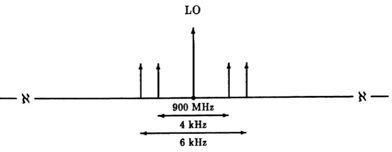
The mobile communication systemuniverse, as illustrated in Fig. 5.2.1, consists of two transmitter galaxies (since adjacent channel interference is of concern there are two transmitters which modulate the information signals up to two

differ-ent carrier frequencies in the adjacdiffer-ent channels), a combiner star, a transmission medium galaxy and a receiver galaxy.

The rest of this chapter is devoted to the functional descriptions of stars which build up the galaxies and finally the universe.

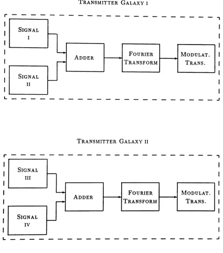
5.3.1

Transmitter Galaxies

In transmitter galaxy I, there are two signal stars as shown in Fig. 5.3.1. Each of the signal stars generates a sinusoidal signal which is the discrete sequence of the sampled analog waveform. The frequency and corresponding sampling rate

TRANSMITTER GALAXY I

- - - ,

-SIGNAL

~ I

...

ADDER

---+ _{TRANSFORM TRANS.}

SIGNAL

-II

r

-L____________________

TRANSMITTER GALAXY II

r - - - -

- - - ,

SIGNAL

-III

~ _{FOURIER MODULAT.}

ADDER

TRANSFORM TRANS.

--..

SIGNAL

-IV

L ~

addition of the two input sample streams. Therefore, each signal star must have

the same sampling rate while generating the sinusoidal waveform. After the adder

star, a two-tone sinusoidal signal is obtained. The two-tone signal was chosen for

its convenience in measuring the intermodulation distortion [54]. Following the

adder star, the time domain two-tone signal is passed through the F FT (Fast

Fourier Transform) star by which the information is transformed into the

fre-quency domain. The next step is to modulate the baseband signal to a higher

frequency suitable for transmission through the channel. This is achieved by the

modulator /translation star which performs double-sideband suppressed carrier

(DSBSC) modulation on the baseband signal [30]. The suppressed carrier

fre-quency and the other parameters are specified in the user-defined CAPSIM

topol-ogy. The description of the transmitter galaxy I I is similar since it consists of

identical blocks as the transmitter galaxy I.

In Fig. 5.2.1, the two transmitter galazy8 are connected to the combiner star.

As its name implies, the combiner star combines the two different spectrums and

sends the resulting RF spectrum through the iransmis sion medium galaxy.

5.3.2

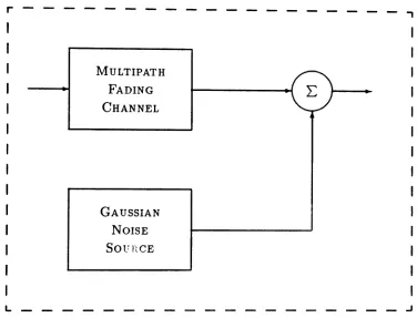
Transmission Medium Galaxy

As mentioned in Chapter 4, the transmission medium gala:cy in Fig. 5.3.2 is a

r - - - _ ,

MULTIPATH

FADING

CHANNEL

GAUSSIAN

NOISE

SOlrnCE

L J

- normalized to the energy in the direct path) are under direct user control.

In addition, the user is allowed to adjust the relative phase

t/J

multipath component relative to the direct path component. Other parameter

choices include the nominal differential delay To and the differential Doppler

/0

associated with the two multipath components. All of these parameters can be

modified through the parameters list in the user-defined CAPSIM topology.

The noise star in the transmission medium galazy is simply a white Gaussian

noise generator operating in the frequency domain. The additive noise components

are the sampled values of white Gaussian noise spectrum. The variance of the

Gaussian noise is a parameter under user control.

5.3.3

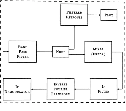
Receiver Galaxy

The receiver galazy, illustrated in Fig. 5.3.3, is composed of a bandpass filter

star, a mizer (FREDA) star, an IF filter siar , a IFFT (Inverse Fast Fourier

Transfonn) star, and an IF demodulator star, The ba,ndpo,~.! filter .ttlr is a

bandpass filter represented in the frequency domain. It has lower and upper

cut-off frequencies and roll-cut-off factor in the transition band which' are specified in the

user-defined CAPSIM topology. Those parameters are effective in the adjacent

channel interference measurements as explained in Section 4.3.2. The RF signal

r _{- - - - - - - -}

---,

FILTERED

RESPONSE PLOT

BAND

~ _MIXER

- - + _{PASS NODE}

(FREDA)

FILTER

--IF

IF

FOURIER ~

DEMODULATOR

TRANSFORM FILTER

L ---~

from the inadequate filtering. The mixer star takes the RF spectrum and invokes

FREDA to analyze the nonlinear RF mixer circuit illustrated in Fig. 4.3.3. The

local oscillator power and the other circuit parameters are specified in the

user-defined FREDA net-list. The output of the mieer sia» is taken by the

IFFT

star which carries out an inverse Fourier transform on the IF frequency spectrum.

Hence, the time domain IF waveform is obtained after the

IFFT

several IF waveforms and spectrums are presented in Chapter 6.

Finally, the IF demodulator star demodulates the IF signal using time domain

techniques. The demodulation techniques are beyond the scope of this work. Thus,