INVESTIGATION
Computationally Ef
fi
cient Sibship and Parentage
Assignment from Multilocus Marker Data
Jinliang Wang
Institute of Zoology, Zoological Society of London, London NW1 4RY, United Kingdom
ABSTRACTQuite a few methods have been proposed to infer sibship and parentage among individuals from their multilocus marker genotypes. They are all based on Mendelian laws either qualitatively (exclusion methods) or quantitatively (likelihood methods), have different optimization criteria, and use different algorithms in searching for the optimal solution. The full-likelihood method assigns sibship and parentage relationships among all sampled individuals jointly. It is by far the most accurate method, but is computationally prohibitive for large data sets with many individuals and many loci. In this article I propose a new likelihood-based method that is computationally efficient enough to handle large data sets. The method uses the sum of the log likelihoods of pairwise relationships in a configuration as the score to measure its plausibility, where log likelihoods of pairwise relationships are calculated only once and stored for repeated use. By analyzing several empirical and many simulated data sets, I show that the new method is more accurate than pairwise likelihood and exclusion-based methods, but is slightly less accurate than the full-likelihood method. However, the new method is computationally much more efficient than the full-likelihood method, and for the cases of both sexes polygamous and markers with genotyping errors, it can be several orders faster. The new method can handle a large sample with thousands of individuals and the number of markers limited only by the computer memory.
O
VER the past few decades, statistical methods have been proposed to infer close relationships such as par-entage and sibship from molecular marker data (Blouin 2003; Jones and Ardren 2003; Jones et al. 2010). They are all based on Mendel’s laws of inheritance (the laws of segregation and independent assortment) to infer the ge-nealogical relationships among individuals from their mul-tilocus genotypes. Some of them employ the laws only qualitatively, excluding a relationship among a set of indi-viduals if their genotypes are incompatible given the rela-tionship under the laws. In an exclusion-based parentage analysis, the parentage of an offspring is assigned to a can-didate if it is the only one that is nonexcluded (Jones and Ardren 2003). In an exclusion-based sibship analysis, a set of individuals are excluded as full siblings if their genotypes cannot be generated from the same pair of parental geno-types at any locus (e.g., Berger-Wolfet al.2007). Exclusion-based methods are appealing because they are simple in concept and implementation, quick in computation, anddo not require allele frequency information. However, exclu-sion methods suffer from several weaknesses.
First, real data sets usually contain genotyping errors, null alleles, and mutations (Pompanon et al.2005), which may lead to false exclusions. Ironically, more data (with more loci and individuals) contain more information but also potentially more errors or mutations, which could result in more false exclusions. Although in principle it is possible to accommodate genotyping errors in exclusion methods (by allowing for a threshold number of mismatches in parentage exclusion analysis, for example), the rule brought in (such as the threshold of mismatches) is arbitrary and rigid and has the danger of false parentage or sibship assignments. Second, the valuable marker information is not fully uti-lized. It is true that allele frequencies for a population are usually unknown and have to be estimated from the sample being analyzed for relatedness. Such estimated allele fre-quencies are usually imprecise due to the small sample sizes and biased due to the relatedness between individuals that is unaccounted for. The problems are severe especially when the sample is small and contains a high proportion of related individuals. However, inaccurately estimated allele frequen-cies could still provide important information for relation-ship inference in likelihood-based methods. Furthermore, it is possible to obtain unbiased allele frequency estimates by Copyright © 2012 by the Genetics Society of America
doi: 10.1534/genetics.111.138149
accounting for relatedness in the same likelihood frame-work. Third, the exclusion rules are necessary but insuffi -cient for relationship inference. For example,mindividuals with the same genotype AA andnindividuals with the same genotype BB are always compatible with (nonexcludable from) a full sibship, because the m+ ngenotypes can be generated by the same pair of parents with a genotype AB. However, applying Mendel’s laws quantitatively, the likeli-hood that thesem+nindividuals are full siblings relative to the likelihood that they come from two full-sib families (one with m individuals of genotype AA and the other with n individuals of genotype BB) diminishes rapidly with an in-creasing value of either morn. Therefore, exclusion-based sibship inference provides a lower bound of the number of sibships and an upper bound of sibship size, but not the optimal sibship assignments. Fourth, exclusion-based meth-ods rely on highly polymorphic codominant markers, and its power diminishes quickly with a decreasing polymorphism of markers. In a full-sibship analysis, exclusion is impossible for biallelic dominant or codominant markers and for any two individuals, no matter how many markers are used and how polymorphic the markers are. Fifth, exclusion methods are applicable to the simplest situation of parentage or full-sibship inference, but are difficult to implement and have diminishing powers for the inference of more remote rela-tionships such as half sibship and of multiple relarela-tionships. More advanced methods employ Mendel’s laws quanti-tatively to calculate the likelihoods of different candidate relationships among a set of individuals and choose the re-lationship that has the maximum likelihood as the best in-ference. These likelihood-based methods largely overcome the above weaknesses of exclusion-based methods, but are more sophisticated and time consuming in computation. The simplest likelihood methods consider the relationship for a pair of individuals in isolation, ignoring all other individ-uals related or unrelated to the dyad. In parentage analysis, for example, the likelihood of each candidate as a parent of a single offspring is calculated and the candidate that has a significantly higher likelihood than the others is assigned parentage of the offspring (Marshall et al.1998; Hadfield et al. 2006). The offspring may have siblings in the sample who share the same parent (or parents), but still it is analyzed in isolation of its siblings. As a result, these pairwise-likelihood methods may create relationships that are in conflict when all individuals are considered jointly and may lead to a loss of power due to the insufficient use of marker data, as explained in Wang and Santure (2009). A more powerful, accurate, and robust approach is to consider the relationships among all individuals in a sample (Painter 1997; Thomas and Hill 2000, 2002; Emery et al. 2001; Smith et al. 2001; Almudevar 2003; Wang 2004; Wang and Santure 2009). Because of the computational complexity, most methods are constrained to the simple case of inferring full sibship in a single cohort sample taken from a species with monogamy for both sexes (e.g., Painter 1997; Smithet al.2001; Thomas and Hill 2000). More recent work
has extended the methods to allow the joint inference of multiple relationships (full and half sibship as well as par-entage) in a two-generation sample (e.g., Emeryet al.2001; Wang and Santure 2009). Although these recent methods are shown to be more powerful,flexible, and robust (Wang and Santure 2009), they are computationally demanding and are constrained to the analysis of small data sets in practice. For a large data set with many individuals and markers, these methods either do not converge (Emery et al. 2001) or take too much time to complete (Wang and Santure 2009). This is unfortunate because currently large data sets can be obtained at a rapidly decreasing cost and effort. With the development of automated high-throughput methods, a sample of hundreds or even thousands of indi-viduals can be genotyped for millions of single-nucleotide polymorphisms (SNPs) at ease. With the sophisticated model of multiple relationships under the polygamous mat-ing systems of both sexes, it is unrealistic for the current methods to analyze such a big data set.
In this article, I develop a new likelihood-based method to infer full and half sibship as well as parentage in a two-generation sample of individuals from marker data. I show by analyzing simulated and empirical data sets that the new method is slightly less accurate than our previous likelihood method (Wang and Santure 2009), but still outperforms many other methods. Importantly, it is computationally much more efficient and can handle large data sets with thousands of individuals genotyped for millions of loci. I describe the method first and then investigate its statistical behavior and accuracy by analyzing some empirical and simulated data sets. The accuracy and computational time of different meth-ods are compared, and the results are discussed.
Methods
Genetic model
A relationship configuration of theN + M + Findividuals consists of a partition of theNoffspring into full-sib and half-sib families and a parentage assignment/unassignment of the Mmales in CFS and of theFfemales in CMS to the inferred families. A configuration therefore specifies the relationships among all individuals in a sample, under the genetic model above. There are many combinatorial configurations, and the aim is to construct and evaluate alternative confi gura-tions and search for the best one that most parsimoniously explains the genotype data. Therefore a relationship infer-ence algorithm must provide a method for evaluating thefit of a configuration to the data and a method for constructing and searching configurations. For the latter task, I use the simulated annealing algorithm, which is a likelihood-guided Monte Carlo method for the construction and search of
con-figurations. This is necessary because it is impossible (but also unnecessary) to enumerate all possible configurations even for a small sample size (say,N= 10 individuals). The algorithm constructs and searches through just a small fraction of all possible configurations that have relatively high likelihood values tofind the best configuration with the maximum likeli-hood. In this article, I use the same simulated annealing algo-rithm for configuration construction and search, as described in Wang and Santure (2009). I introduce a new and compu-tationally efficient method for configuration evaluation only so that large data sets can be handled.
Configuration score
The most time consuming part of our previous likelihood method (Wang and Santure 2009) is the calculation of the likelihood of a configuration. The computational cost increases roughly exponentially with the size of a sibship structure, determined roughly by the numbers and mating patterns of contributing male and female parents, exponentially with the number of alleles per locus, and linearly with the number of markers. For a cluster of many interconnected full-sib fam-ilies contributed by a large number of fathers and mothers, the computational cost is huge because likelihoods must be computed and summed over all possible parental genotype combinations for each locus. Ifnparents contribute to a clus-ter of offspring and each parent has mfeasible genotypes, then the number of parental genotype combinations is mn.
The value of mis small for a marker without typing errors and mutations or with few alleles, but is large for a marker with many alleles when typing errors are accounted for.
To reduce computation, I must abandon the idea of using the likelihood of a configuration to measure its plausibility. Instead, I use the sum of the log likelihoods between all pairs of individuals given their relationships in a confi gura-tion as the score of plausibility. Let gli and glj be the
ge-notypes of offspring i and j (i, j =1, 2, . . ., N) at locus l (l= 1, 2,. . ., L), and Roij be the relationship (full sibs, half
sibs, or non-sibs) betweeniandj. GivenRo
ij and the
popula-tion allele frequencies, the log probability of the multilocus genotypes of offspringiandjisQo
ij= PL
l¼1LnðPrðgli;gljjRoijÞÞ.
Similarly, the log probability of the multilocus genotypes of
candidate malei(i=1, 2,. . .,M) and offspringjgiven their relationshipRm
ij (father–offspring or unrelated) and the
pop-ulation allele frequencies is Qm
ij ¼ PL
l¼1LnðPrðgli;gljjRmijÞÞ.
The log probability of the multilocus genotypes of candidate femalei(i=1, 2,. . .,F) and offspringjgiven their relation-shipRf
ij (mother–offspring or unrelated) and the population
allele frequencies is Qf
ij¼ PL
l¼1LnðPrðgli;gljjRfijÞÞ. The
likeli-hood score for a configurationCis then defined as
SðCÞ ¼X N
i¼1 XN
j¼iþ1
Qoijþ XM
i¼1 XN
j¼1
Qmij þ XF
i¼1 XN
j¼1
Qfij: (1)
In (1), Qo
ij,Qmij, and Qfij can be calculated for any given
re-lationship (full sibs, half sibs, parent–offspring, or unrelated) between individualsiandj, taking into account the two pos-sible types of genotyping errors (allelic dropouts and other errors including mutations) as in Wang and Santure (2009). Note that the likelihood score as defined in (1) is similar to that of Smithet al.(2001). The main difference is that their likelihood score is the sum of the logarithms of likelihood ratios between all pairs of individuals and thus applies to the simplest case of only two alternative relationships, which are full sibs and unrelated. The use of likelihood rather than likelihood ratio makes the method more general, applicable to the joint inference of multiple relationships. Another dif-ference is that (1) accounts for genotyping errors, while the likelihood score in Smithet al.(2001) was calculated assum-ing perfect genotype data without errors.
To further reduce computation, I compute and store an upper triangle matrix ofN(N–1)/2 values ofQo
ij between all
pairs of offspring for the halfsib relationship, a similar matrix for the fullsib relationship, and a vector ofNvalues, which are the log probability of the multilocus genotype of each offspring given allele frequencies. I also compute and store an M·N matrix of values of Qm
ij between each candidate fatheri and
offspringjfor the parent–offspring relationship and a vector of Mvalues, which are the log probability of the multilocus geno-type of each candidate father given allele frequencies. Similarly, a matrix and a vector are calculated and stored for candidate mothers. All these matrixes and vectors just need to be calcu-lated once (if allele frequencies are not updated) and are used repeatedly in calculating (1) for different configurations.
In the simulated annealing algorithm, a new configuration is generated by modifying part of an old one. The modified part usually involves one or just a few individuals. This implies that, to obtain the likelihood score of a new configuration, we can use the score of the old configuration and just update the pairwise-likelihood values involving those individuals who are in the modified part of the configuration. This procedure also reduced computational burden substantially.
Simulated annealing algorithm
frequencies. When a sample contains few families of highly variable sizes, allele frequencies calculated from the sample under the assumption that all individuals are unrelated will be imprecise and biased. The frequencies of alleles observed in large and small families will be over- and underestimated, respectively. The biased allele frequencies will bias likeli-hood calculations, decreasing the likelilikeli-hood of large families and increasing the likelihood of small families. Conse-quently, large families tend to be split into two or more small families in reconstruction. To infer relationships accurately, allele frequencies should be recalculated using the inferred parental genotypes and their probabilities periodically in the simulated annealing algorithm (Wang and Santure 2009), and the updated allele frequencies are used in subsequent likelihood calculations. This iterative procedure has been proven to be effective, but is unfortunately unsuitable for the likelihood-score (LS) method. This is because confi gura-tions are evaluated and accepted or rejected on the basis of their pairwise-likelihood scores in simulated annealing, while parental genotypes and their probabilities are based on the full likelihood of configurations in updating allele frequencies. The adoption of two different statistical frame-works leads to poor convergence of the simulated annealing algorithm (data not shown). I use the following procedure of multiple runs to update allele frequencies and improve relationship inference when a sample is suspected to contain both very large and very small families.
Multiple runs (say, five) are conducted in tandem for a data set, and each run updates relationship configurations only in simulated annealing. The frequencies of all alleles at a locus are assumed to be equal in the first run and are estimated from the best configuration of the previous run using the full-likelihood method in the following runs. The optimal relationship configuration and allele frequencies from the last run are returned as the best estimates. Therefore, updating allele frequencies requires multiple runs and thus increases computational time by several-fold compared with a single run without allele frequency updating. In practice, updating allele frequencies should be opted for only when a sample is suspected to contain few families with highly variable sizes. In the analyses of empirical and simulated data sets shown below, allele frequencies are not updated to save computational time.
Evaluation of the Method
To understand the performance and robustness of the new method, it is applied to simulated and empirical data sets in which genealogical relationships among sampled individu-als are known. It is individu-also compared with some previous methods for the accuracy of relationship inference and for computational efficiency.
Other methods for comparison
I focus on comparing the new LS method with the commonly used pairwise-likelihood methods and our full-likelihood
method for sibship and parentage inferences. Several other methods developed specifically for full-sibship reconstruc-tion are also compared in analyzing some empirical data sets.
Pairwise-likelihood (PL) methods calculate the probabil-ity of the marker data of a pair of individuals (dyad) under each of a number of candidate relationships as the likelihood of the relationship, and the inferred relationship is the one with the maximum likelihood (e.g., Epstein et al. 2000; McPeek and Sun 2000). In this study, I assume that the candidate relationships are full sibs, half sibs, and unrelated under polygamy and are full sibs and unrelated under mo-nogamy, for sibship inference among individuals in OFS. The procedure of Marshall et al. (1998) in determining the D statistic to resolve parentage with a certain level of confi -dence is adopted for parentage inference. Parentage assign-ments are made and accepted at the confidence level of 95%. Both pairwise methods for sibship and parentage assignments are implemented in the software Colony2 (http://www.zsl. org/science/research-projects/software/), which is used in analyzing simulated and empirical data sets (below).
Our full-likelihood (FL) method for the joint inference of sibship and parentage was described in Wang and Santure (2009) and was implemented in Colony2. There are a num-ber of options (such as running length, numnum-ber of runs, sibship prior) of using this method, and the defaults as-sumed in Colony2 are used in analyzing the data in this study.
An exclusion-based full-sibship analysis method was de-veloped by Berger-Wolf et al.(2007). The method employs a deterministic combinatorial optimization method to assign all sampled individuals into the smallest number of full-sib families, which conform qualitatively to Mendel’s laws of inheritance at multiple marker loci. The method (called combinatorial algorithm, CA) is implemented in a web-based program KINALYZER (http://kinalyzer.cs.uic.edu/), which is used in analyzing the empirical data sets in this study.
Another exclusion-based full-sibship analysis method was proposed by Butler et al. (2004). It attempts to maximize Simpson’s index of concentration while imposing a full-sib genotype constraint from Mendel’s laws. Similar to the combinatorial method briefed above, the method effec-tively searches for the partition that has the smallest num-ber of full-sib families. The original algorithm of Butler et al. (2004) was improved for computational efficiency by Konovalov et al. (2004) and implemented in the software KinGroup (http://www.kingroup.org). This improved algo-rithm (MS2 hereafter) is used in analyzing the empirical data sets in this study.
families one by one, and the addition order is implemented via the descending ratio search algorithm that takes individ-uals from pairs with the clearest relationships (highest likeli-hood ratios). The DR method as implemented in KinGroup is used in analyzing the empirical data sets in this study.
Empirical data sets
Different pedigree reconstruction algorithms are tested and compared on several empirical data sets with known family structures.
A salmon data set: Taken from a genetic improvement program of the Atlantic salmon federation (Herbingeret al. 1999), the salmon data set is composed of 759 individuals in 12 full-sib families whose sizes are 8, 10, 31, 51, 54, 59, 64, 69, 75, 91, 107, and 140. Each individual is genotyped at four microsatellite loci, which have 8, 10, 11, and 14 ob-served alleles in the sample. The data set is cleaned, con-taining no missing genotypes and no apparent mutations and genotyping errors as checked against the known paren-tal genotypes. This data set or its subsets have been ana-lyzed several times by previous methods (e.g., Smith et al. 2001; Butler et al. 2004;Berger-Wolf et al. 2007) and are ideal for exclusion-based methods because they have large family sizes, contain no known genotyping errors, and have highly polymorphic codominant markers. In this study, the accuracy of different methods is compared on analyzing this data set.
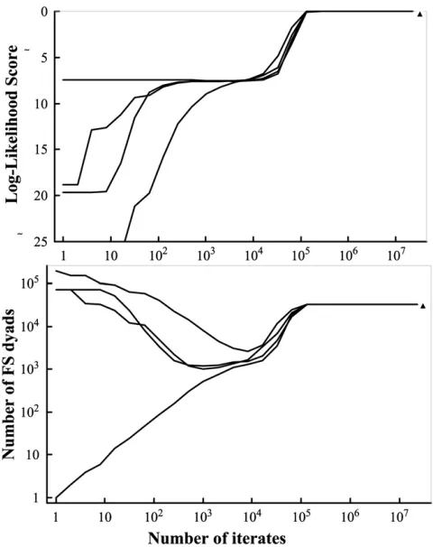
The data set was also used to test the convergence of the new LS method. For this purpose, four runs of the data set were conducted with different starting configurations and random number seeds, assuming a small error rate (0.001) for each locus. The four initial configurations are: (1) all 759 individuals are in a single full-sib family, (2) each individual is in a distinctive full-sib family, (3) thefirst 380 individuals are in a single full-sib family and each of the remaining 379 individuals is in a distinctive full-sib family, and (4) the last 380 individuals are in a single full-sib family and each of the remaining 379 individuals is in a distinctive full-sib family. The changes in likelihood and number of full-sib dyads of the configurations as functions of iterates in the simulated annealing algorithm are plotted and compared among the four runs.
An ant data set: The ant data set is from a study on the mating frequency of an ant species, Leptothorax acervorum (Hammondet al.2001). It consists of 377 ant workers (dip-loid) sampled from 10 known colonies (full-sib families), with each of 6 colonies contributing 45 workers and the remaining 4 colonies contributing 47, 44, 9, and 7 workers to the sample. The workers were genotyped at up to six microsatellite loci, which have a number of observed alleles varying between 3 and 22. This data set has a substantial proportion of missing genotypes and contains a few geno-typing errors as identified in a previous analysis (Wang 2004). Therefore a small error rate (0.01) for both allelic
dropouts and false alleles at each locus was assumed in the analyses by the FL and LS methods implemented in Colony2. The DR method could account for genotyping errors, while all the other methods are exclusion based and assume per-fect data.
A human data set:A subset of CEPH data (available online
http://www.cephb.fr/en/cephdb/) used in this study con-tains an OFS sample of 343 offspring taken from 59 families with known parents and some known grandparents. The full-sibship size (number of full sibs) in the OFS sample varies from 1 to 12, with the corresponding counts of {1, 4, 4, 8, 13, 9, 7, 4, 4, 2, 2, 1}. The subset also contains 105 candidate fathers in a CFS sample and 119 candidate moth-ers in a CMS sample. The actual fathmoth-ers and grandfathmoth-ers of the 59 families are included in the CFS sample if they have genotypes missing at most at one of the five highly poly-morphic SSR loci used in the analyses. Mother candidates are selected similarly. Note that grandparents are included in the candidate parent samples to increase the difficulty in parentage analyses because they compete with the actual parents for parentage assignments.
The data are analyzed assuming monogamy for both sexes, a probability of 0.5 that the parent of an offspring is included in the candidate parent sample and no genotyping errors. Allele frequencies are assumed unknown and calcu-lated from the three samples, assuming all individuals are unrelated. The genotypes of sampled individuals atfive SSR loci are used by FL and LS methods for the joint sibship and parentage analyses, by PL, CA, MS2, and DR for sibship analysis and by PL for parentage assignments. To check the convergence of the FL and LS methods for this data set, both
five and three SSRs are used in different replicate runs with different starting configurations and random number seeds.
Simulations
The new method is thoroughly tested and compared with other methods by analyzing extensive simulated data gen-erated under various scenarios. The simulation encompasses various full- and half-sib family structures and size distri-butions, varying sample sizes and marker information contents, and parentage assignments for sibling families of various sizes.
a half-sib family. For example, 16(5, 5) means there are 16 half-sib families, and each family comprises 2 full-sib families (each having 5 full siblings) resulting from a com-mon father mated with two different mothers. Ten markers, each having 10 codominant alleles, are used in sibship analyses.
Simulation 2 considers the effect of marker information content. A simulated OFS consists of 100 individuals whose true full-sib configuration is 10(1, 2, 3, 4). The number of microsatellites varies between 2 and 20, while the number of SNPs varies between 20 and 100. Each microsatellite and SNP is assumed to have 10 and 2 codominant alleles, respectively.
Simulation 3 considers the effect of sample size, sibship structure, and genotyping errors on the accuracy and com-putational time of different methods. A set of 10 markers, each having 10 codominant alleles, was used to infer the sibship structure of an OFS of various sizes and sibship types. For the case of full sibship (both sexes monogamous), an OFS contains 8, 16, 32, 64, 128, 256, or 512 sets of full-sib families, each set having a true full-sib configuration (1, 2, 3, 4). For the case of half sibship, an OFS contains 5, 10, 20, 40, 80, 160, or 320 families. Each family consists of 16 offspring, with each offspring coming from each of the 16 possible matings between 4 males and 4 females. For both cases, therefore, sample sizes vary between 80 and 5120. Each of the 10 markers is assumed to have an error rate of either 0 or 0.01 for both allelic dropouts and false alleles. These error rates are used in simulating and analyzing data.
Simulation 4 considers the accuracy of parentage as well as sibship assignments. Five sets of full-sib families, each having a true full-sib configuration of (1, 2, 3, 4, 5, 6, 7, 8), were included in an OFS (180 individuals), while the 5·8 = 40 mothers as well as 160 unrelated candidate mothers are included in a CMS. Candidate fathers are assumed unavail-able. Each sampled individual (180 in OFS and 200 in CMS) was genotyped at 5 or 10 microsatellite loci, each having 10 alleles. Maternity assignments were made by FL, LS, and PL methods, assuming a prior probability that a true mother is included in CMS is 0.95.
In each simulation, the frequencies of alleles at each locus were drawn from a uniform Dirichlet distribution. The mul-tilocus genotype of each parent was then generated using the allele frequencies, assuming no linkage among loci, Hardy–Weinberg, and linkage equilibria. The multilocus ge-notype of each offspring is generated from those of its parents, following Mendelian segregation. To simulate mis-typings in simulation 3, offspring phenotypes are obtained by changing their genotypes at a given error rate (0.01) following the allelic dropout and false allele models. For each parameter combination, 100 replicate data sets are simulated and analyzed, except when the offspring sample size is .160. For simulations with an OFS of 320, 640, 1280, 2560, and 5120 individuals, the replicates are 80, 60, 40, 20, and 10, respectively. For the cases of both sexes
polygamous, FL was applied to data sets only when an OFS has 640 or fewer individuals.
Measurement of accuracy
I measure accuracy by the statistic, P(a|b), the frequency of dyads assigned relationshipawhen their actual relationship is b(Thomas and Hill 2000; Wang 2004). For sibship inference among the offspring, accuracy is measured by P(FS|FS), P(HS|HS), andP(UR|UR), where FS, HS, and UR are full sibs (FS), half sibs (HS), unrelated offspring (UR). I also measure the overall accuracy by the total number of incorrectly inferred dyads or the frequency of correctly inferred dyads. For parent-age inference, accuracy is measured by the frequencies that parentage is correctly assigned,P(PO|PO), or correctly unas-signed,P(XO|XO), when the actual parent is included in and excluded from the candidate pool, respectively. An advantage of using these separate measurements instead of a single one (such as the partition distance; Gusfield 2002) is that they are indicative of not only the accuracy, but also the causes of the inaccuracy (e.g., whether FS is inferred as HS) where the re-lationship reconstruction is imperfect.
Results
Analysis results of empirical data sets
The salmon data set:The results in Table 1 show that the FL method reconstructs the sibship structure of the 759fish perfectly, with the relationship among all individuals being correctly identified. The LS method partitioned the 759fish into 12 full-sib families. While the majority of these families are correctly reconstructed, a few are split or merged. In total, 1280 unrelated and 484 full-sib dyads were
misspeci-fied by LS as full-sib and unrelated dyads respectively, result-ing inP(FS|FS) = 98.47% andP(UR|UR) = 99.50%. MS2 and DR methods overestimated the number of full-sib fam-ilies by 1 and 2, respectively. On the basis of pairwise rela-tionships, MS2 is slightly more accurate and DR is less accurate than LS for this data set. The total number of pair-wise relationships incorrectly identified by MS2, DR, and LS is 1089, 3119, and 1764, respectively. The PL method does not attempt to reconstruct family structures but just esti-mates pairwise relationships. It performs very poorly com-pared with other methods.
Table 1 does not list the results from the CA method. It assigned the 759fish into 12 full-sib families. However, each of 7fish appears in 2 families, resulting in a total number of 766 individuals (i.e., with seven duplications) appearing in the configuration. This is obviously an unfeasible confi gura-tion, although the relationships among most individuals are correctly identified. Because of the presence of duplicated individuals, it is difficult to count the numbers of correctly identified full-sib and unrelated dyads and to compare its performance with the other methods as done in Table 1.
the likelihood scores (and any statistics of the inferred confi g-uration such as the number of full-sib dyads) of the four runs converge to the same value at iterates105. The maximum log-likelihood score of the best configuration,27608110.1, is larger than the value for the true configuration which is 27608831.6. The reason that the LS method does not render the true configuration as its best solution is not because the method fails to find the true configuration but because it is inferior to the best solution in terms of likelihood score. This is not surprising given that the data set has only four microsatellites and, among the 759fish, there are only 521 unique multilocus genotypes and 1206 pairs of individuals have identical multilocus genotypes. More marker information is needed for LS to completely reconstruct the family structure of this data set.
The ant data set:Both LS and FL methods reconstructed the sibship structure of this data set perfectly without any error (Table 2). Multiple runs with different initial configurations and random number seeds as done for the salmon data set yield exactly the same results for both methods. MS2, DR, and PL methods have a similar accuracy, resulting in incor-rect relationship inference for hundreds of dyads. The sib-ship configuration rendered by CA is again unfeasible and self-contradictory. While two individuals are missing from the configuration, 18, 2, 1, and 1 individual appear in 2, 3, 4, and 5 full-sib families, respectively. Therefore, a total number of 404 individuals appear in the configuration, in-stead of the actual number of 377.
The human data: For sibship analyses of this data set, FL and LS are the most accurate methods, which give no misassignments, MS2 is slightly less accurate, while PL and DR have the lowest and much reduced accuracy (Table 3). CA yielded an unfeasible configuration in which each of three individuals appears twice. For parentage analyses, FL and LS produced perfect results while PL yielded 77 misas-signments. Close inspection of these misassignments show that most errors are false assignments in which the grand-parents instead of true grand-parents are assigned parentage. The LS and FL methods do not make the same mistake as the PL method because they consider parentage assignments for an entire sibship rather than a single offspring. The probability that a grandparent has a higher likelihood as a parent of a sibship than a true parent decreases rapidly with an
in-creasing sibship size. This is also true for candidates less or not related to the true parents. When siblings are present in OFS, it is generally more powerful to make joint sibship and parentage assignments as in the LS and FL methods than to make parentage assignments for a single offspring as in PL methods.
Results from multiple runs of the data set with different starting configurations and random number seeds show that both the FL and LS methods converge reliably to the same configuration. However, when only three of thefive loci are used in the analyses, both methods no longer converge consistently (data not shown). Nonetheless, the different Table 1 Accuracy of different methods for sibship assignments of the salmon data set
Method No. FS family No. dyads FS|UR No. dyads UR|FS P(FS|FS) P(UR|UR)
MS2 13 240 849 0.9731 0.9991
DR 14 1,818 1,301 0.9588 0.9929
PL — 14,327 6,135 0.8058 0.9441
LS 12 1,280 484 0.9847 0.9950
FL 12 0 0 1.0000 1.0000
The actual numbers of full-sib families, full-sib dyads, and unrelated dyads are 12, 31,588, and 256,073, respectively. Column 2 gives the inferred number of full-sib families. Columns 3 and 4 list the numbers of unrelated and full-sib dyads that are inferred as full sibs and unrelated, respectively. Columns 5 and 6 list the frequencies that full-sib and unrelated dyads are inferred as such, respectively.
best configurations rendered by different runs of the LS (or FL) method have very similar likelihood scores and have a very similar accuracy. Increasing the length of the runs reduces but does not solve the problem. The nonconver-gence is probably caused by the existence of numerous configurations that have the same or very similar likelihood scores, which hinders the simulated algorithm to move to the configuration with the global maximal likelihood score.
Simulation results
The analyses of empirical data sets above and simulations show that the LS method is not less accurate than the exclusion (e.g., MS2, CA) and pairwise-likelihood (e.g., DR)-based full-sibship reconstruction methods even in situations that are most favorable to the latter (e.g., large sibship, few highly polymorphic codominant markers, no genotyping errors). Furthermore, the LS method has a much wider ap-plication scope and can be applied to dominant and codom-inant markers with 2 or more alleles, data with and without genotyping errors, the assignments of full and half sibship, as well as parentage, diploid and haplodiploid species, dioecious and monoecious with and without inbreeding. Therefore, in the simulations below, I concentrate on com-paring the accuracy and computational efficiency of FL, LS, and PL methods only.
Family structures: The actual familial structure of the individuals in a sample has a large impact on the perfor-mances of LS and FL methods, but little impact on the performance of PL method (Table 4). Under otherwise the same conditions, large and simple families are generally easier to infer than small families or families with a complex genetic structure (e.g., many full-sib families nested in many interconnected half-sib families) by LS and FL methods. In contrast, the accuracy of PL method is little affected by the
actual family size and structure. This is understandable be-cause LS and FL methods consider the relationship among all individuals simultaneously, while PL considers the rela-tionship of each pair of individuals in isolation.
Table 4 shows that LS is much more accurate than PL but is less accurate than FL for all three full-sib family structures. The reduction in accuracy of LS relative to FL increases with an increasing size and complexity of the actual sibship struc-ture in a sample. The table also shows that, with the same marker information, both the FL and LS methods have no-ticeably lower accuracy for the smallest family structures FS160(1) and HS80(1, 1).
It becomes more challenging to infer half siblings for all three methods, because half sibship is intermediate in re-latedness between full sibship and unrelated. When marker information is insufficient, it is difficult to distinguish HS from FS and UR. LS performs much better than PL, but is now substantially less accurate than FL. Most of the errors made by LS are the confusions between relationships similar in relatedness, mistaking FS as HS and HS as UR, or vice versa mistaking HS as FS and UR as HS. However, there is no systematic bias toward any relationship, with each type of error occurring at roughly the same frequency. In terms of the absolute number of errors, however, most errors occur to the most frequent true relationship. If there are many more FS than HS dyads in a sample, for example, then most errors would be FS misspecified as HS. With an increase in marker information, however, the accuracy of the LS method quickly improves, similar to the full-sib case shown in Figure 2.
Note that with half-sib structure HS80(1, 1), it seems as if PL outperforms LS and FL performs the worst, when evaluated by P(HS|HS) and P(UR|UR). However, we need to realize that different types of dyads (FS, HS, UR) occur in dramati-cally different frequencies. In terms of the total number of correctly inferred dyads, the order of the accuracy of the three Table 2 Accuracy of different methods for sibship assignments of the ant data set
Method No. FS family No. dyads FS|UR No. dyads UR|FS P(FS|FS) P(UR|UR)
MS2 10 381 509 0.9366 0.9939
DR 10 374 58 0.9928 0.9940
PL — 879 27 0.9966 0.9860
LS 10 0 0 1.0000 1.0000
FL 10 0 0 1.0000 1.0000
The actual numbers of full-sib families, full-sib dyads, and unrelated dyads are 10, 8,024 and 62,852, respectively. The columns are the same as those of Table 1.
Table 3 Accuracy of different methods for sibship and parentage assignments of the human data set
Method
No. FS family
No. dyads FS|UR
No. dyads UR|FS
No. dyads PO|P
No. dyads
PO|X P(FS|FS) P(UR|UR) P(PO|PO) P(XO|XO)
MS2 62 46 68 — — 0.9319 0.9992 — —
DR 48 682 176 — — 0.8236 0.9882 — —
PL — 2290 66 69 8 0.9339 0.9603 0.8930 0.8049
LS 59 0 0 0 0 1.0000 1.0000 1.0000 1.0000
FL 59 0 0 0 0 1.0000 1.0000 1.0000 1.0000
methods is reversed. There are far more UR dyads (12640) than half-sib dyads (80) for this simulated sibship structure, and it isP(UR|UR) that determines the overall accuracy.
Marker information:The results from simulation 2 (Figure 2) show that the accuracy of FL, LS, and PL methods improves with an increasing number of microsatellite or SNP loci. While FL and LS always perform much better than PL, FL is sub-stantially more accurate than LS only when marker informa-tion is scarce. When there are.10 microsatellites or 60 SNPs, the difference in performance between FL and LS is hardly detectable. Figure 2 also shows that roughly 60 SNPs are equivalent to 10 microsatellites (each having 10 alleles) in information content and can be used to obtain almost perfect sibship reconstruction for this simulated sibship structure. This microsatellite and SNP equivalence depends on allele fre-quency distributions of both markers and on the applications. For estimating effective population size from linkage disequi-librium, for example, roughly 90 SNPs are equivalent to 10 microsatellites in information content (Waples and Do 2010). For more complicated sibship structures or many small sib-ships, however, more markers are needed to obtain highly accurate sibship assignments.
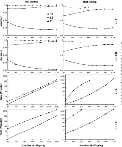
Sample size and genotyping error: For both the full- and half-sibship cases, markers with and without genotyping er-rors, and across all of the sample sizes, the most, least, and intermediate accurate methods are FL, PL, and LS, respectively. While the difference between FL and LS is small in general, PL yields much worse sibship assignments than FL and LS. Genotyping errors, at a rate of 0.01, have little effect on the accuracy of FL and LS, but do reduce the accuracy of PL. This is because genotyping errors can be identified and corrected for in relationship inference with an increasing power as more relatives are considered jointly. While PL considers a pair of individuals in isolation, both FL and LS consider all individuals in a sample.
For computational time, PL is very fast and its running time is not shown in Figure 3 for comparison. The running time of both FL and LS increases log linearly with the loga-rithm of offspring sample sizes. For the case of full sibship, FL runs only slightly slower than LS whene= 0 (no geno-typing errors), but takes roughly 10 times the computational time of LS whene= 0.01. This is also true for the case in which one sex is monogamous and the other sex is
polyga-mous (data not shown). At a higher mistyping rate, the difference in running time between FL and LS becomes even greater. For the case of half sibships in which both sexes are polygamous, the computational time of the FL method is several orders longer than LS, no matter for markers with or without genotyping errors. Therefore, analyses of samples with.640 individuals whene= 0 or 320 individuals when e= 0.01 were not conducted by the FL method. For LS, it is interesting to note that mistypings do not increase the com-putational time in the full-sibship case, but does increase the computational time substantially in the half-sibship case. This is because, although mistypings do not alter the cost of likelihood score calculation, they lead to many more com-peting configurations with a similar likelihood score and Table 4 Accuracy of FL, LS and PL methods for different family structures
FL method LS method PL method
Sibship
structure P(FS|FS) P(HS|HS) P(UR|UR) No.
error P(FS|FS) P(HS|HS) P(UR|UR) No.
error P(FS|FS) P(HS|HS) P(UR|UR) No. errors
FS160(1) — — 0.9939 78 — — 0.9914 109 — — 0.9702 379
FS16(10) 1.0000 — 1.0000 0 0.9979 — 0.9996 7 0.9445 — 0.9825 250
FS2(1,2,3,4, 10,20,40) 1.0000 — 1.0000 0 0.9989 — 0.9994 8 0.8933 — 0.9900 226
HS80(1,1) — 0.1924 0.9810 305 — 0.2466 0.9745 382 — 0.6855 0.8559 1846
HS16(5,5) 0.9972 1.0000 1.0000 1 0.8503 0.8815 0.9945 161 0.8090 0.6634 0.8883 1536
HS8(1, 2,3,4,10) 0.9963 0.9988 1.0000 5 0.8585 0.8828 0.9972 343 0.7886 0.6303 0.9109 1794
The columns No. errors list the total number of dyads whose relationships are incorrectly inferred among 12,720 dyads in a sample of 160 individuals.
thus result in more searching time in the simulated anneal-ing algorithm. For FL, mistypanneal-ings always increase computa-tional time enormously irrespective of the sibship structure.
Parentage assignments: The accuracy of maternity assign-ments increases with sibship size for the FL and LS methods, but stays the same for the PL method (Figure 4). This is because both FL and LS methods infer sibship and maternity jointly. When two or more offspring are inferred to share the same mother, they provide more information about their mother and thus allow for more accurate maternity assignment than when a single offspring is considered alone for its maternity inference as is the case for the PL method. While FL invariably outperforms the other two methods, LS becomes better than PL
when the number of siblings is two or more, depending on the marker information. When siblings are suspected to be frequent in OFS, it is advisable to use FL or LS for parentage assignments. Note that maternity assignments shown in Figure 4 were carried out in a situation favorable to the PL method, which is most powerful when parents are completely sampled. It is even more outperformed by the FL and LS methods when just a small fraction of the parents are sampled and included in the candidate lists (data not shown).
Discussion
In this article I proposed a new method, the LS method, to make sibship and parentage assignments from marker data, and investigated its accuracy and computational efficiency Figure 3 Accuracy and compu-tational time of different meth-ods as a function of offspring sample sizes. Ten markers (each having 10 alleles in a uniform fre-quency distribution) with (e ¼
in comparison with other methods using both empirical and simulated data. The new method can be regarded as an in-termediate (or compromise) between the pairwise-likelihood method, which considers the relationship between each pair of individuals in isolation, and the full-likelihood method, which considers the relationship among all individuals in a sample jointly. The LS method is similar to FL, but uses the sum of the pairwise log likelihood as a score to measure the plausibility of a relationship configuration.
There are several advantages of the new method, and some of these have been demonstrated in this article. Compared with exclusion-based methods, the LS method applies to a much wider range of situations. It can be used to infer full sibship, half sibship, and parentage jointly and can use dominant, codomi-nant markers (SNPs or microsatellites), and a combination of them. Compared with PL methods, it uses marker information more efficiently because it considers the relationship among all individuals in a sample and thus provides more accurate sibship and parentage assignments as verified by simulated and empirical data sets. Furthermore, all inferred relationships are guaranteed to be consistent, while the PL method may yield pairwise relationships that are in conflict when put together. Compared with the FL method, LS has the great advantage of computational efficiency, which makes it feasible to handle large data sets involving many loci and many individuals. Computa-tion is becoming an increasingly important issue currently; more
and more large data sets can be generated with relative ease thanks to the development in molecular biology.
The main disadvantage of LS is that it is less accurate than FL, especially when marker information is scarce and the family structure in a sample is weak or complicated. This is not unexpected as the likelihood score defined in (1) is an approximation based on the assumption that dyads are independent of each other. Compromising between accuracy and computational feasibility, I suggest that FL be used when at least one sex is monogamous or when the offspring sample size is small. In such a case, LS is not much faster but is noticeably less accurate than FL, except when the number of marker loci is large. When both sexes are polygamous and the offspring sample size is large, however, we may have to use the LS method as the computational burden for the FL method is unrealistically too high. This is especially true when markers having mistypings are used in the analysis.
Analyses of empirical and simulated data indicate that the LS method is well behaved and converges reliably when marker information is not too scarce. Even when the method does not converge, the suboptimal configurations rendered are usually very close to each other and to the optimal one in both the likelihood score and the inferred relationships. When marker information is insufficient, there could be many configurations with a similar or the same likelihood score, which hinders the convergence of the simulated annealing algorithm. In such a case, it is unrealistic and also probably unnecessary to pursue absolute convergence. The LS method is fast because the log likelihoods of each possible candidate relationship for each pair of individuals are calculated only once and stored and reused repeatedly in calculating the score of a configuration. Genotyping errors at each locus can be accounted for with no extra computa-tional cost. The computacomputa-tional time of the likelihood score of a configuration is not affected by the number of loci, while the total running time decreases actually with an increase in the number of markers because of the reduction in the number of configurations with a similar or the same likelihood scores. As shown in the simulated and empirical data, LS is quite successful in inferring various complicated family structures using a widely variable number and polymorphic levels of markers. It also works well for vastly different sample sizes and for different marker types (e.g., dominant markers, SNPs). Sup-porting the findings of Smith et al. (2001), however, the LS method is sensitive to allele frequency misspecifications. Allele frequencies, when estimated from a sample of individuals dom-inated by a few large families by assuming unrelatedness, are inaccurate, with frequencies of those alleles appearing in large (small) families overestimated (underestimated). When these estimates are used in sibship inference, large families tend to be split (data not shown). In such a case, the iterative approach proposed in this study improves greatly the accuracy of relation-ship analysis, because allele frequencies are improved iteratively by accounting for the reconstructed family structures. In prac-tice, one may know nothing about the family size distribution before a sibship analysis. In such a situation, one can take a two-Figure 4 Accuracy of parentage assignments of the FL, LS and PL
step process. First, the data are analyzed without updating allele frequencies. Second, if few families with highly variable sizes are reconstructed, then one needs to rerun the data with allele frequency updated; otherwise, the results of the first analysis are accepted.
The LS method, like any other methods used in relation-ship inference, makes many assumptions that may not be met in reality. For example, it assumes Hardy–Weinberg and linkage equilibrium and no linkage at marker loci, the absence of noncandidate relationships (e.g., cousins), and random mating. However, violations of these assumptions usually have small effects on the accuracy of FL, as checked by my previous study (Wang 2004). This is also likely to be true for the LS method, as it performed very well for the three empirical data sets that may not satisfy these assump-tions. Examining these factors systematically by simulation for the LS method is out of the scope of this study.
The LS method developed herein reconstructs a one- or two-generation pedigree from marker data. It is notable that some progress has been made with the more general problem of reconstructing pedigrees of greater depth. To make com-putation feasible, current models are usually specialized or constrained to loop-free pedigrees of individuals sampled from a hermaphrodite annual species with partial selfing (e.g., Wilson and Dawson 2007), to pedigrees of complex relation-ships among genotyped individuals but only relatively simple relationships among ungenotyped ancestors (e.g., Almudevar 2003), or to a very small sample of individuals from a popula-tion with known mating systems (e.g., Gasbarra et al.2007). Further developments in these methods to remove the restric-tions (assumprestric-tions) would be highly desirable and exciting.
Acknowledgments
I thank C. M. Herbinger for sending me his salmon data set and M. A. Beaumont, C. M. Herbinger, R. Waples, and an anonymous referee for valuable comments on earlier versions of this manuscript.
Literature Cited
Almudevar, A., 2003 A simulated annealing algorithm for maximum likelihood pedigree reconstruction. Theor. Popul. Biol. 63: 63–75. Berger-Wolf, T. Y., S. I. Sheikh, B. DasGupta, M. V. Ashley, I. C. Caballero
et al., 2007 Reconstructing sibling relationships in wild popula-tions. Bioinformatics 23: I49–I56.
Blouin, M. S., 2003 DNA-based methods for pedigree reconstruc-tion and kinship analysis in natural populareconstruc-tions. Trends Ecol. Evol. 18: 503–511.
Butler, K., C. Field, C. M. Herbinger, and B. R. Smith, 2004 Accuracy, efficiency and robustness of four algorithms allowing full sibship reconstruction from DNA marker data. Mol. Ecol. 13: 1589–1600. Emery, A. M., I. J. Wilson, S. Craig, P. R. Boyle, and L. R. Noble, 2001 Assignment of paternity groups without access to
paren-tal genotypes: multiple mating and developmenparen-tal plasticity in squid. Mol. Ecol. 10: 1265–1278.
Epstein, M. P., W. L. Duren, and M. Boehnke, 2000 Improved inference of relationship for pairs of individuals. Am. J. Hum. Genet. 67: 1219–1231.
Gasbarra, D., M. Pirinen, M. J. Sillanpää, E. Salmela, and E. Arjas, 2007 Estimating genealogies from unlinked marker data: a Bayesian approach. Theor. Popul. Biol. 72: 305–322.
Gusfield, D., 2002 Partition-distance: a problem and class of per-fect graphs arising in clustering. Inf. Process. Lett. 82: 159–164. Hadfield, J. D., D. S. Richardson, and T. Burke, 2006 Towards un-biased parentage assignment: combining genetic, behavioural and spatial data in a Bayesian framework. Mol. Ecol. 15: 3715–3730. Hammond, R. L., A. F. G. Bourke, and M. W. Bruford, 2001 Ma-ting frequency and maMa-ting system of the polygynous ant, Lep-tothorax acervorum. Mol. Ecol. 10: 2719–2728.
Herbinger, C. M., P. T. O’Reilly, R. W. Doyle, J. M. Wright, and F. O’Flynn, 1999 Early growth performance of Atlantic salmon full-sib families reared in single tanksvs.in mixed family tanks. Aquaculture 173: 105–116.
Jones, A. G., and W. R. Ardren, 2003 Methods of parentage anal-ysis in natural populations. Mol. Ecol. 12: 2511–2523. Jones, A., M. Clayton, K. Small, A. Paczolt, and N. Ratterman,
2010 A practical guide to methods of parentage analysis. Mol. Ecol. Res. 10: 6–30.
Konovalov, D. A. C. M., and M. T. Henshaw, 2004 KINGROUP: a program for pedigree relationship reconstruction and kin group assignments using genetic markers. Mol. Ecol. Notes 4: 779–782. Marshall, T. C., J. Slate, L. E. B. Kruuk, and J. M. Pemberton, 1998 Statistical confidence for likelihood-based paternity in-ference in natural populations. Mol. Ecol. 7: 639–655. McPeek, M. S., and L. Sun, 2000 Statistical tests for detection of
misspecified relationships by use of genome-screen data. Am. J. Hum. Genet. 66: 1076–1094.
Painter, I., 1997 Sibship reconstruction without parental informa-tion. J. Agric. Biol. Environ. Stat. 2: 212–229.
Pompanon, F., A. Bonin, E. Bellemain, and P. Taberlet, 2005 Ge-notyping errors: causes, consequences and solutions. Nat. Rev. Genet. 6: 847–859.
Smith, B. R., C. M. Herbinger, and H. R. Merry, 2001 Accurate partition of individuals into full-sib families from genetic data without parental information. Genetics 158: 1329–1338. Thomas, S. C., and W. G. Hill, 2000 Estimating quantitative
ge-netic parameters using sibships reconstructed from marker data. Genetics 155: 1961–1972.
Thomas, S. C., and W. G. Hill, 2002 Sibship reconstruction in hierarchical population structures using Markov chain Monte Carlo techniques. Genet. Res. 79: 227–234.
Wang, J., 2004 Sibship reconstruction from genetic data with typing errors. Genetics 166: 1963–1979.
Wang, J., and A. W. Santure, 2009 Parentage and sibship infer-ence from multilocus genotype data under polygamy. Genetics 181: 1579–1594.
Waples, R. S., and C. Do, 2010 Linkage disequilibrium estimates of contemporary Ne using highly variable genetic markers: a largely untapped resource for applied conservation and evo-lution. Evol. Appl. 3: 244–262.
Wilson, I. J., and K. J. Dawson, 2007 A Markov chain Monte Carlo strategy for sampling from the joint posterior distribution of pedigrees and population parameters under a Fisher–Wright model with partial selfing. Theor. Popul. Biol. 72: 436–458.