Dynamic Behaviour of Rigid Pavement Plate due to Load Moving with Acceleration

Dynamic Behaviour of Rigid Pavement Plate

due to Load Moving with Acceleration

Ridwan Halim1, Sofia W. Alisjahbana2

Faculty of Engineering, Department of Civil Engineering, Tarumanagara University, Jakarta, Indonesia 1

Tarumanagara University, Jakarta, Indonesia2

ABSTRACT:Rigid pavement structure is found in many industrial buildings, especially on road structure. Most of the time, road is bypassed by heavy vehicles such as trucks with heavy loads. So, engineer have to design precisely so that structure could meet both the strength and serviceability (deflection) requirements. The rigid pavement dynamic analysis in this thesis is modeled as a concrete plate with boundary conditions of all edges of the plate having semi rigid support and supported by Pasternak foundation model with elastic vertical spring support and continuous shear layer underneath. Transversal loads that cross the plate surface are dynamic load with initial speed and stable acceleration. The load is modeled as a single centered axis load equivalent to the variation of trucks such as Colt Diesel Double (CDD) Los Bak, Colt Diesel Double (CDD) Long Box, dan Colt Diesel Double (CDD) Bak. In this study will also be analyzed various types of parameters such as the value of vehicle coefficient, damping ratio value, and various supporting soil conditions are soft soil, medium soil, and hard soil. Solving the problem of dynamic plate with semi rigid conditions using Modified Bolotin Method (MBM) with two transendental equations. In solving these dynamic functions load we are using special characters of Dirac-delta function. The analysis is performed when the load is above the plate (0 ≤ t¬ ≤ t0), and the final result obtained is the response spectrum or critical speed of the vehicles and forces including moment and shear forces.Introduction

KEYWORDS:MBM (Modified Bolotin Method), semi rigid, dynamic respons, transversal load, acceleration, Pastenak, Dirac-delta, rigid pavement.

I. INTRODUCTION

Plate structures that are often used on roads are rigid pavement structures (concrete layers) and flexible pavement structures (asphalt layers). Rigid pavement is considered to provide several advantages compared to roads using flexible pavement because it can be used on subgrade conditions which has a low or no uniform carrying capacity and rigid pavement is able to withstand heavy loads and spread the force that occurs efficiently towards the subgrade. In 1964, Kerr introduced the simplest elastic foundation model (the Winkler foundation model) [1]. The supporting soil layer is modeled as a supporting spring layer that is spread evenly along the plate. But this model only applies to uniform loads because there is no account of the connection between the layers of soil so as to produce uniform deformation along the plate [2].

One of the foundation modeling that produces a fairly good value and approaches the actual situation is proposed by Pasternak or known as Pasternak's foundation model. Pasternak modeled the supporting soil layer into 2 layers, namely the sliding layer and the spring layer under the plate. Several studies have been conducted based on this foundation modeling, including rigid hardness analysis placed on the supporting soil layer using Pasternak's foundation model and burdened with running loads [3].

constant speed with asymmetrical placement on all sides of the plate, so that the solution to the homogeneous differential equation of the system needs to be solved by Modified Bolotin Method [2]. This method is a numerical method for solving various plate equations through trigonometric functions. This method is superior because it can produce solutions for various types of placement and produce accurate solutions to a high range of vibrations. For semi-rigid placement plates, wave numbers are expressed as pπ / a and qπ / b, with p and q being real numbers that can

be known through two auxiliary problems.

II. LITERATURE SURVEY

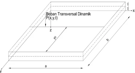
Plates are one of the important parts of a structure in the form of a three dimensional object with a flat and straight surface. One dimension is the thickness is smaller than the other two dimensions namely width and length [5]. As a structural element that plays a role in channeling loads from both lateral (in-plane) and transverse loads. The transverse load that occurs on both static and dynamic plates works perpendicular to the plate surface as shown in Figure 1.

Fig 2:Plate geometry [5]

III.METHODOLOGY

The purpose of this study was to determine the effect of moving loads on rigid pavement plates on deflection, moment, shear, and knowing the critical velocity values due to moving loads with acceleration.

General analysis

The equation of motion of an orthotropic plate loaded by dynamic loads and supported by Pasternak elastic foundation can be expressed by Equation (1).

D ∂ w (x, y, t)

∂x + 2B

∂ w (x, y, t)

∂x ∂y + D

∂ w (x, y, t)

∂y +γh

∂w (x, y, t)

∂t +ρh

∂ w (x, y, t)

∂t −k w−

G ( , , )+ ( , , ) = p(x, y, t) (1)

First auxiliary equation

The solution to the first auxiliary problem is an equation of the position function as follows in Equation (2).

X(x) = cosh + ( ( ) )

( ) sinh −cos −

( ) ( )

( ) sin (2)

Where :

F = D β

ab − D

q b

F = D p

a + D

q a C = cosh πβ

b c = cos (pπ)

S = sinh πβ b

s = sin (pπ) (3)

Second auxiliary equation

The solution to the second auxiliary problem is an equation of the position function as follows in Equation Y(y) =

cosh + ( ( ) )

( ) sinh −cos −

( ) ( )

( ) sin (4)

Where :

θ= (qa) +G (ab)

π D +

2B(pb) D

F = D θ

ab − D

p a

F = D q

b + D

p a C = cosh πθ

a c = cos (qπ)

S = sinh πθ a

s = sin (qπ) (5)

Homogeneous solution

Homogeneous solution, wH,, from the equation of motion according to Equation (1) can be obtained from differential equations which can be expressed as:

(6)

Particular solution

Particular solutions (wP) can be obtained by using the variable separation method. The coefficients contained in the homogeneous solution are expanded according to the influence of the excitation forces that do not yet exist in a homogeneous solution which can be stated as follows:

wH = w(x, y, t) = Wpq(x, y)Tpq(t)

∞

q=1

∞

p=1

wH= w(x, y, t) = Xpq( )Ypq( ) e− ωpq _{0[pq ]}cos[ωD] + _{0[pq ]}sin[ωD] ∞

q=1 ∞

p=1

wp= Xpq(x)Ypq(y)

∞

q=1

∞

p=1

=





                                    







1 ( ) .

. 1 ) ( ) ( . . ) , , 9 2 2 ) ( . 0 0 0 dt t Sin e dy y Y dx x X Q h t y x P pq pq t b y pq a x pq pq z t pq          (7) Total solution

After a homogeneous solution and a particular solution are obtained, thus the total system solution can be expressed as w = wH + wPwhere wH is in accordance with equation (6) and wP is in accordance with equation (7) which can be expressed as:









                                                     









        _{ }        _                         d t Sin e dy y Y Q h t y x P e e b e a e y Y x X t y x w a x pq pq pq pq z t t t t i pq t t i pq t t n pq pq m pq pq pq pq pq 0 2 2 . . 0 . . ) ( 1 . 0 ) ( 1 . 0 ) .( . 1 1 ( 1 1 ) ( . . ) , , ( . . . ) ( ). ( ) , , ( 0 2 0 2 0 (8)

Dynamic load function

The transverse load passing over the surface of the plate can be expressed by the Dirac-delta function as follows in Equation (9):

P (x, y, t) = P[x(t), y(t), t] = P(t).δ[x−x(t)].δ[y−y(t)](9)

Where:

P(t) = Dynamic load acting on the plate which is a t function = P0 (1 + α.Cos[ωt])(10)

P0 = The function of the load position in the direction of average center load and the equivalent load of the vehicle wheel (equivalent single axle laod, ESAL) [kN]

x(t) = Function of load position in x direction = V t + a t

a = The length of the plate in x direction [m] b = The width of plate in y direction [m] Ac = Transverse load acceleration [m/det2] v0 = Transverse load speed[km/jam]

y(t) = Function of load position in y direction [m] =

α = Vehicletypecoefficient

ω = Harmonious load frequency[rad/det]

δ[.] = Dirac’s delta function

By substituting equation (9) into equation (10) and by entering the function of the load position the equation is obtained:

P(x, y, t) = P (1 +αcos[ωt]).δ x−x V t + a t .δ[y− ](11)







 











                                                           











         _{ }        _       b y pq pq pq a x pq t pq t t t i pq t t i pq t t n pq pq m d t Sin e dy y y y Y dx Acc V x x x X Q h Cos P e e b e a e y Y x X t y x w pq pq pq pq pq 0 2 2 . . 0 0 2 0 0 0 . . ) ( 1 . 0 ) ( 1 . 0 ) .( . 1 1 ) ( 1 1 . ). ( . . . 2 1 . ). ( . . . 1 . . . ) ( ). ( ) , , ( 0 2 0 2 0                        (12)

The partial integral in equation (12) can be stated as follows:

(13)

Because of the function of load motion in direction x = V t + a t is a function of time, then equation (12) becomes:







 







. ) ( 1 1 . . . 2 1 . . . . ) ( . . 1 . . . . ) ( ). ( ) , , ( 1 2 2 . . 0 2 0 0 . . ) ( 1 . . 0 ) ( 1 . . 0 ) ( . 1 0 2 0 2 0







         _{ }        _                                                                     m pq pq t pq pq t w t t w i pq t t w i pq t t w n pq pq d t Sin e Acc Vo X Q h y Y Cos P e e b e a e y Y x X t y x w pq pq pq pq pq                   (14)

IV.RESULT AND ANALYSIS Size and material properties of plate

In this study we will discuss the completion of the orthotropic plate dynamic response burdened with the transversal load running as shown in Figure 2 below.

Fig 2:Plate illustration with dynamic transverse load

X_pq(x).δ x−x V_oτ+1 2acτ

2 a

x=0

Y_pq(y).δ[y−y₀] b

y=0

= V_oτ1

2acτ 2 _Y

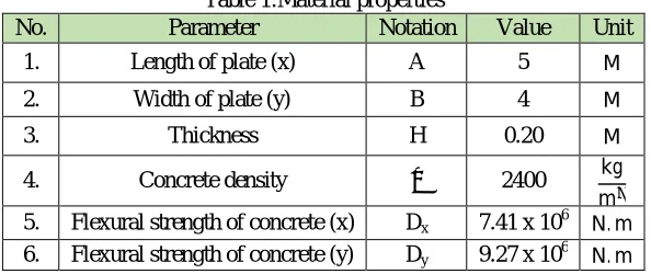
The research data used in the numerical analysis are presented in Table 1.

Table 1:Material properties

No. Parameter Notation Value Unit

1. Length of plate (x) A 5 M

2. Width of plate (y) B 4 M

3. Thickness H 0.20 M

4. Concrete density Ρ 2400 kg

m

5. Flexural strength of concrete (x) Dx 7.41 x 106 N. m 6. Flexural strength of concrete (y) Dy 9.27 x 106 N. m

The research data on transversal load (vehicle load) is attached to Table 2.

Table 2:Transversal load

No. Parameter Notation Value Unit

1. Centralized vehicle load Po 75000 – 140000 N

2. Load frequency ωb 100

rad det

3. Load coefficient α 0.333 - 0.667

4. Vehicle speed v0 60

km jam

5. Accelartion Ac 2

m det

In this study also involved soil as a medium found below the base of the slab. Soil support is modeled continuously along the bottom of the plate [4]. The value of the spring constant k and the shear constant Gs Pasternak can be seen in Table 3.

Table 3:Spring constant k dan shear constant Gs of Pasternak Foundation Tye of Soil

Constant Unit Soft Soil Medium Soil Hard Soil

K

MN

27.2 54.4 108.8

Gs

MN

Case study

In this study several variations of cases were taken based on the parameters described in Table 4 as follows:

Table 4:Variations in research case studies

Case

A B H Po Acc Alfa

ζ

K Gs

Annotation

[m] [m] [m] [kN] [m/det2] [α] [MN/m/m2] [MN/m]

1 A

5 4 0,2 80 2 0,5 0.05

- - TanpaLapisan Tanah

B 27,2 9,52 Lapisan Tanah Lunak

C 54,4 19,04 Lapisan Tanah Sedang

D 108,8 38,8 Lapisan Tanah Keras

2 A

5 4 0,2 80 2 0,5 0

27,2 9,52 Soft soil layer

B 0.05

C 0.1

3 A

5 4 0,2 80 2

1/3

0.05 27,2 9,52 Soft soil layer

B 1/2

C 2/3

4 A

5 4 0,2 75

2 0,5 0.05 27,2 9,52 Soft soil layer

B 80

C 140

III.3. Results and discussion

Based on the case variation table above, the analysis is carried out to get the final result in the form of maximum absolute deflection, critical speed, and forces in the structure.

Table 5:Absolute maximum deflection case study [1] – [4]

Absolute Maximum Deflection

Case Absolute Maximum Deflection Time

[m] [s]

1

A 0.00269 0.057

B 0.00091 0.040

C 0.00068 0.052

D 0.00035 0.056

2

A 0.00132 0.039

B 0.00091 0.040

C 0.00070 0.041

3

A 0.00093 0.040

B 0.00091 0.040

C 0.00089 0.063

4

A 0.00085 0.040

B 0.00091 0.040

C 0.00159 0.040

study was 0.2 m, so that the deflection permit was 0.02 m. It can be concluded based on the Table 5 that of all variations of case studies.

The case study used to get the maximum response sought by speed consists of 4 main case studies, namely the comparison of the strength of the supporting plate, the damping ratio, the coefficient of load, and the type of truck that passes. The critical speed absolute deflection for case study [1] & [2] studied was measured at the center of the plate can be seen in Table 6.

Table 6:Absolute deflection of critical speed – Case [1] & [2]

Speed (V)

Absolute Deflection of Critical Speed

[1A] [1B] [1C] [1D] [2A] [2B] [2C]

Wihout Base Soil Soft Soil Medium Soil Hard Soil ζ = 0% ζ = 5% ζ = 10%

[Km/Hour] [m] [m] [m] [m] [m] [m] [m]

40 0.003456 0.001376 0.000763 0.000491 0.001801 0.001376 0.001166

48 0.003362 0.001223 0.000803 0.000490 0.001650 0.001223 0.001031

56 0.002963 0.000943 0.000740 0.000406 0.001347 0.000943 0.000790

64 0.002390 0.000908 0.000607 0.000332 0.001323 0.000908 0.000694

72 0.002106 0.000870 0.000539 0.000309 0.001260 0.000870 0.000737

80 0.002283 0.000880 0.000549 0.000323 0.001137 0.000880 0.000805

Minimum 0.002106 0.000870 0.000538 0.000309 0.00105 0.00087 0.00069

Maximum 0.003456 0.001376 0.000803 0.000491 0.00192 0.00138 0.00117

The critical speed absolute deflection for case study [3] & [4] studied was measured at the center of the plate can be seen in Table 7.

Tabel 7:Absolute deflection of critical speed – Case [3] & [4]

Speed (V)

Absolute Deflection of Critical Speed

[3A] [3B] [3C] [4A] [4B] [4C]

α= 0.333 α= 0.5 α= 0.667 P0 = 75 kN P0 = 80 kN P0 = 140 kN

[Km/Hour] [m] [m] [m] [m] [m] [m]

40 0.001206 0.001376 0.001547 0.001290 0.001376 0.002409

48 0.001071 0.001223 0.001376 0.001147 0.001223 0.002141

56 0.000910 0.000943 0.001061 0.000884 0.000943 0.001649

64 0.000928 0.000908 0.000888 0.000851 0.000908 0.001588

72 0.000891 0.000870 0.000883 0.000816 0.000870 0.001523

80 0.000811 0.000880 0.000960 0.000825 0.000880 0.001541

Minimum 0.00081 0.00087 0.00088 0.00082 0.00087 0.00152

Moments and shear forces can be calculated according to Kirchoff's small deflection theory as follows:

2 2

x x 2 y 2

w w

Momen m = D + ν

x y

  

 _{ }

 

 

(15)

2 2

y y 2 x 2

w w

Momen m = D + ν

y x

  

 _{ }

 

 

(16)

2 2

x x 2 2

w w

Gaya geser q = D + B

x x y

 

  

 _{ }

 _   _

(17)

2 2

y y 2 2

w w

Gaya geser q = D + B

y y x

 

  

 _{ }

 _   _

(18)

Equation 15 to Equation 17, the bending moment of the x and y directions is the second derivative of the deflection function w (x,y,t) In addition, deflection of function w (x,y,t) if it is lowered three times the sehar force will be obtained on the x and y axes.The parameter of this at initial positionx( )= V t + a t andy( )= .

V. CONCLUSION

Based on the results of the analysis carried out in this study, some conclusions can be taken as follows:

1. One of the factors that causes an increase in the value of the natural frequency of the structure is the condition of the plate supporting soil. In this study 3 types of supporting soil were studied, namely soft soil, medium soil, and hard soil. Based on the results of the analysis it was found that the higher the carrying capacity of the soil, the resulting structure will become stiffer so that both the deflection and the inner force produced are smaller.

2. The maximum deflection that occurs in case study 1A is the maximum deflection among all case studies, with

the absence of supporting soil layers. This is because the load frequency (ωb) = 100 rad / sec passing which is adjacent to the system's natural frequency (ωn) = 162,393 rad / sec.

3. The effect of speed on the dynamic response of the system for case studies [1] and [2]. Critical speeds that produce maximum dynamic deflection varies from 40 - 48 km / h and speeds of 64 - 88 km / h are critical speeds that produce minimum dynamic deflections. Maximum dynamic deflection occurs in case 2A with a value of 0.001916 m (this value is only around 10% of the deflection permit of 0.02 m). For case studies [3] and [4] shows that the speed of 40 km / h is the critical speed that produces the maximum plate dynamic deflection and the speed of 72 km / h is the critical speed of the system which causes the minimum plate dynamic deflection.

4. Based on the results of internal force analysis for each case it can be concluded that, for case 4 show that the greater transverse load that passes on the road (P0), the greater the moment and shear values produced, while if the greater the carrying capacity of the soil, the value of the damping ratio (ζ), and vehicle type coefficient (α),

the smaller the moment value and shear produced.

REFERENCES

1. Kerr, A. D., “A Study of New Foundation Model”, Acta Mechanica, Springer-Verlag, 1964.

2. Alisjahbana, S. W. dan Wangsadinata, W., “Dynamic Response of Rectangular Orthotropic Plate Supported by Pasternak Foundation Subjected to Dynamic Load”, First International Structural Specialty Conference, Calgary, Alberta, Canada, 2006.

3. Zaman, E. A., “Dynamic analysis of concrete pavements resting on a two parameter medium”, 1993.

4. Baadilla, Douglas Abdullah., “Dinamika Pelat Perkerasan kaku dengan Tahanan Tepi Sembarang”. Disertasi Doktor Teknik Sipil, Pascasarjana Universitas Tarumanagara, Jakarta, 2006.

5. Szilard, R., “Theory and Analysis of Plates : Classical and Numerical Methods”, Prentice Hall, Inc., New Jersey, 1974.

6. Bolotin, V. V., “The Edge Effect in The Oscillations of Elastic Shells”. PMM, Vol. 24, No. 5, 1960, Moscow, Rusia, pp. 831-843, 1960. 7. King, Wilton W., “Applications of Bolotin’s Method to Vibrations of Plates”. AIAA Journal, Vol. 12, No. 3, March 1974, pp. 399-401, 1974. 8. Paz, Mario., “Structural Dynamics : Theory and Computation Second Edition”, Chapman & Hall, New York, 1985.

New Jersey, USA, 2004.

10. Timoshenko, S. P., and Goodier, J. N., “Theory of Elasticity”, International Student Edition, McGraw-Hill Book Company, Singapore, 1974. 11. Alisjahbana, S. W., Wangsadinata, W., dan Baadilla, D. A., “Dynamic Behaviour of Rigid Concrete Pavements Under Dynamic Traffic Loads”.

1st International of European Asian Civil Engineering Forum, Jakarta, 2007.