ABSTRACT
SHIAU, YO-JIN. Greenhouse Gas Emissions and Carbon Sequestration Potential of a Created Tidal Marsh. (Under the direction of Dr. Michael R. Burchell II).
Along with other ecosystem services that wetlands provide, carbon sequestration in
wetlands through accumulated plant biomass can potentially make these ecosystems net
carbon sinks. This ecosystem service can potentially be beneficial to remediate the rising
global carbon dioxide concentrations in the atmosphere and provide additional economic
benefits to wetland restoration projects. However, the dynamic of accumulated biomass
(carbon input) and greenhouse gas (GHG) fluxes (carbon outputs) in wetlands have not been
well studied in brackish salt marshes with salinities > 20 ppt. This research was conducted to
provide a clearer understanding of how pore water salinity and other environment factors
found in created salt marshes impact GHG fluxes, how diel CO2 flux varied in a created
brackish salt marsh, and whether carbon sequestration can be considered a significant
ecosystem service provided by created brackish salt marshes.
Beginning in March 2011, a GHG study was conducted over a 33 month period at a
four year old created tidal salt marsh in Carteret County, North Carolina. GHG samples were
collected using a replicated static chamber method within three distinct plant zones (S.
alterniflora, J. roemerianus and S. patens). Along with GHG gas sampling, pore water salinity, temperature, conductivity and soil redox potential were measured at the same
frequency. Soil pore water samples were collected seasonally to analyze the available sulfate
and nitrate concentrations in the rhizosphere. Beginning in March 2013, continuous CO2
flux monitoring experiments were conducted in the marsh using an infrared gas analyzer
biomass harvesting events and aboveground and belowground litter bag studies were
conducted in the 2013 growing season to estimate the carbon storage rates in the same marsh.
Results from the manual chamber study showed pore water salinity was in the
hypothesized range of 20 – 30 ppt. The major source of GHG emissions from the marsh was
CO2 and ranged from -48 – 192 mg C m-2 hr-1, which was near the lower end of other
wetland types with lower salinities. The CH4 and N2O fluxes appeared to be lower than other
studies, with ranges of -0.33 – 0.86 mg C m-2 hr-1 and -0.11 – 0.10 mg N m-2 hr-1,
respectively. Results also showed marsh vegetation adaptations to wetland conditions may
affect the oxidation status (reflected to different redox values) in the rhizosphere and may
indirectly affect soil microbial activities and GHG production.
The major GHG emission from the created brackish marsh was CO2. Continuous
measurements showed diel CO2 flux appeared to be tied to tidal fluctuations. A model was
developed to simulate these daily fluctuations based on soil temperature and site hydrology.
The effect of these daily fluctuations appeared to be small when yearly flux was estimated,
because the annual simulated CO2 flux rate for the site was within the range estimated using
the manual static chamber method. The small differences between the monthly gas sampling
and continuous flux monitoring, and the wide variations from the CO2 flux survey indicated
the temporal variation was less important than the spatial variation in CO2 flux. While the
continuous CO2 flux measurements was beneficial to observe and understand the diel
variations of CO2 flux, the estimated annual CO2 flux was similar to the rate estimated using
the manual static chamber method.
carbon sink because of the high plant primary production and low GHG emissions. In the
long term, 23 – 53 % of the stored carbon was degraded and stored as soil carbon pool.
Overall, the 14 ha created marsh would reduce around 281 tons CO2eq of the global warming
potential and could bring $3232 dollars worth of the carbon credits to global carbon markets
based on the carbon balance data in the 2013 growing season. While the economic returns of
carbon sequestration do not alone justify the expense of creating tidal marshes, it does add to
the sum of other economic benefits such as fisheries, storm protection, water treatment, and
© Copyright 2014 Yo-Jin Shiau
Greenhouse Gas Emissions and Carbon Sequestration Potential of a Created Tidal Marsh
by Yo-Jin Shiau
A dissertation submitted to the Graduate Faculty of North Carolina State University
in partial fulfillment of the requirements for the degree of
Doctor of Philosophy
Biological and Agricultural Engineering
Raleigh, North Carolina
2014
APPROVED BY:
________________________________ ________________________________ Dr. Michael R. Burchell Dr. Stephen W. Broome
Committee Chair Minor Representative
________________________________ ________________________________ Dr. François Birgand Dr. Owen W. Duckworth
DEDICATION
I would like to dedicate this dissertation to my family, from whom I have got unconditional
BIOGRAPHY
Yo-Jin Shiau was born on February 19, 1982 to Shing-Gwo Shiau and Hsuen-Ling
Wang. He grew up in Taipei, the capital city of Taiwan with his parents and two sisters.
Because of his father's work in marine geology modeling, he started to learn computer
programming since he was six years old. Since then, computer programming became a part
of his life for his entertainment.
After graduation from the Affiliated Senior High School of National Taiwan Normal
University in 2000, Yo-Jin enrolled in National Taiwan University in Bioenvironmental
Systems Engineering (former name: Agricultural Engineering) with an idea of becoming a
modeler in bioinformatics. In the summer of 2002, before started the junior year of his
undergraduate study, he had a chance to serve as a guide in a series of ecological tours led by
Dr. Wen-Lian Cheng and held by the Mandarin Daily News. He introduced the environment,
ecology, and social culture to kids aged 7 to 12 years old. At the same time, he was able to
rethink his career goals and decided to change his study focus to the environmental
protection and remediation. He joined Dr. Cheng's ecological engineering Lab during his
master's study in Fall 2004 and developed a non-invasive environmental monitoring
technique for treatment wetlands and streams.
After his graduation, he served for the compulsory community service in the
Environmental Protection Administration, Taiwan during 2007 – 2008. He received the
Government Scholarship to Study Abroad in 2009 from the Ministry of Education, Taiwan,
ACKNOWLEDGMENTS
Thanks to my advisor, Dr. Michael Burchell. It was extremely fortunate for me to have
such a supervisor, who always had time for me, and taught me so much in every aspect of
science, from experimental design to data analysis, from critical thinking to scientific
writing. I cannot have asked for a better supervisor.
Thanks to my committee members, Dr. Francois Birgand, Dr. Steve Broome, Dr. Owen
Duckworth and Dr. Ken Krauss for all their inputs from the experiment designs, data analysis,
result interpretations and scientific writing. This dissertation would not have been completed
without their suggestions and encouragement. I would also like to thank Dr. Jason Osborne
at NC State University Department of Statistics who helped me on the statistical model in
Chapter 2.
I especially want to thank Rebecca Moss and Nicole Cormier for analyzing the gas
samples and the DEA samples. Also because of their help on the instrument setup, my field
experiment was able to be completed.
I also want to thank Rachel Huie and Hiroshi Tajiri at NC State University Department
of Biological and Agricultural Engineering for analyzing the pore water samples, and Lisa
Lentz at the Department of Soil Science for analyzing the plant tissue samples.
The three year field experiments were extremely time and labor consuming. They
could have only been accomplished due to the help from different people. I want to thank Dr.
Randall Etheridge, who helped me accomplished almost all of the field trips in the past three
Fernandez, Nicki Dobbes, Taylor Barto, Molly Mikan, Ryan Hutcherson, Ian Cader, Megan
Fruchte, Jamie Blackwell, and Carolyn Currin for all their effort on the experiments involved
in this dissertation.
This research study would not have been accomplished without the funding from the
USGS National Wetland Research Center. In addition, my 4.5 years of the Ph.D. study in the
U.S. was made possible because of a scholarship funded by Ministry of Education, Taiwan
for the first two years.
It would not be possible of me to finish my study abroad without family support. I
want to thank to my family in Taiwan sharing all the pressure and frustration during my Ph.D.
study. I also want to thank my wife and my daughter spent all their time to stay in the U.S.
and support me in the past 4.5 years. Because of my wife's excellent painting skills, some of
the graphs in this dissertation can be presented exquisitely.
TABLE OF CONTENTS
LIST OF TABLES ... xi
LIST OF FIGURES ... xiii
CHAPTER 1: Introduction and Literature Review ... 1
Introduction ... 1
Greenhouse effect and global warming ... 1
Characteristics of greenhouse gases ... 1
Wetlands and global warming ... 3
Soil microbial respiration and GHG production ... 4
Importance of sulfate in soil greenhouse gas emissions ... 6
Other potential environmental factors that influence GHG emissions ... 11
Methods of soil greenhouse gas sampling ... 13
Importance of blue carbon to climate change ... 15
Research objectives ... 18
References ... 19
CHAPTER 2: Greenhouse gas emissions in a created brackish salt marsh in eastern North Carolina ... 32
Abstract ... 32
Introduction ... 33
Materials and Methods ... 37
Site description ... 37
Greenhouse gas flux measurements ... 38
Other environmental measurements ... 42
Litter bag study ... 43
Soil denitrification enzyme activities ... 44
Statistical analyses ... 45
Environmental parameters ... 46
Greenhouse gas measurements ... 51
Litterbag studies ... 55
Soil denitrification enzyme activity ... 57
Discussion ... 58
Conclusions ... 67
References ... 68
CHAPTER 3: Modification and application of a soil respiration model to predict diel CO2 emission in a tidally influenced brackish marsh in Eastern North Carolina ... 74
Abstract ... 74
Introduction ... 76
Materials and Methods ... 79
Site description ... 79
Continuous carbon dioxide measurement ... 81
Soil CO2 efflux survey measurement ... 83
Development of soil respiration model for a tidal system ... 85
Technique for filling data gaps ... 87
Results and Discussion ... 88
Initial simulations using nested Q10 model ... 94
Model simulations: Separating diurnal and nocturnal data ... 98
Model simulations: seasonal hysteresis effects ... 99
Improvement of the nested Q10 model with tidal marsh specific conditions ... 101
Model test: Q10 model to reflect tidal influence ... 106
Comparison of the nested Q10 model and the tidally influenced Q10 model ... 107
Simulated annual soil respiration rates ... 110
Limitations of the tidally influenced Q10 model ... 112
Conclusion ... 113
CHAPTER 4: Carbon sequestration and soil carbon accumulation in a recently created
brackish marsh in Eastern North Carolina ... 122
Abstract ... 122
Introduction ... 123
Materials and methods ... 126
Site description ... 126
Carbon output measurement ... 128
Carbon input measurement ... 128
Plant carbon and nitrogen contents ... 131
Biomass decomposition experiment ... 132
Estimates of the carbon storage rate and the soil carbon content ... 132
Net global warming potential reduction in the created marsh ... 134
Results ... 135
Carbon output from the brackish marsh ... 135
Plant biomass accumulation in the brackish marsh ... 135
Plant carbon and nitrogen contents ... 137
Plant decomposition rates in the marsh ... 139
Plant net primary production, net global warming potential reduction, and soil carbon accumulation rate in the created brackish tidal marsh ... 139
Discussion ... 142
Plant net primary production in coastal marshes ... 142
Soil carbon accumulation rate in the created brackish tidal marsh ... 146
Economic benefits of the net global warming potential reduction in the brackish tidal marsh ... 148
Conclusion ... 151
References ... 152
CHAPTER 5: Conclusions ... 159
APPENDICES ... 163 Appendix A: Original greenhouse gas flux and environmental factor data in the studied tidal brackish marsh ... 164 Appendix B: Original greenhouse gas flux data in the brackish marsh ... 190 Appendix C: The linear relationship graphs for fitting the missing data ... 199 Appendix D: Calculation of the potential influence of tidal fluctuations on soil CO2 flux .. 206
Appendix E: The original continuous CO2 flux data in the studied tidal brackish marsh .... 208
Appendix F: Simulated CO2 flux data using the tidally influenced Q10 model in the studied
LIST OF TABLES
Table 1.1. Different pathways of methanogenesis ... 6
Table 1.2. Sulfate reducing reactions produce carbonic acids ... 8
Table 1.3. Summary of the GHG fluxes in previous research ... 10
Table 1.4. Carbon storage rate and carbon stock in different ecosystems ... 17
Table 2.1. The average elevations where static chambers were located using North American Vertical Datum of 1988 (NAVD88) as the reference sea level elevation. ... 38
Table 2.2. Concentrations of the standard gases for calibrating the gas chromatograph. ... 41
Table 2.3. Summary of data collected for the GHG experiment. ... 43
Table 2.4. Seasonal soil pore water nitrate and sulfate concentrations at different locations in North River Farm created salt marsh. (The "Low", "Mid" and "High" represented the lowest, the middle and the highest elevations in one replicate block) ... 51
Table 2.5. Summary of seasonal mean and regression results for GHG fluxes of CO2, CH4 and N2O fluxes. ... 52
Table 2.6. Comparison of the GHG fluxes results with research in different salinity ranges. 60 Table 2.7. Soil denitrification potential rates from freshwater and saltwater wetlands. ... 66
Table 3.1. The equations of different soil respiration models ... 77
Table 3.2. The values of the parameters from different simulations using nested Q10 model and the tidally influenced Q10 model. ... 108
Table 4.1. Summary of aboveground biomass in the created and natural marsh in March and August 2013. ... 136
Table 4.2. Summary of belowground biomass in the created and natural marshes in March and August 2013. ... 137
Table 4.3. The carbon and nitrogen contents in the aboveground and belowground tissues of three plants. ... 138
Table 4.5. The summary of the plant NPP, the plant carbon production, the effective carbon storage, and the soil carbon storage rate in the studied brackish tidal marsh. ... 140
Table 4.6. Comparison of the aboveground and belowground net primary production (NPP) of the three plants in different research sites in east coasts of America. ... 142
Table 4.7. Comparison of the daily accumulation rate of soil carbon in different types of ecosystems. ... 147
Table 4.8. The globally potential annual carbon credits in seven ecosystems and the expected annual benefit for per dollar of construction/restoration costs. ... 150
Table D1. The raw greenhouse gas fluxes and environmental factor data in the studied tidal brackish marsh during 2011 – 2013 ... 164
Table E1. The original CO2 flux data measured using the infrared gas analyzer in the studied
brackish marsh in 2013 ... 213
LIST OF FIGURES
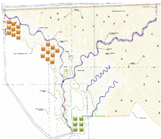
Fig. 2.1. The locations of the GHG static chambers in the upstream and downstream locations in the created marsh (indicated as orange squares), and further downstream in the reference marsh (indicated as green squares). ... 39 Fig. 2.2. The cross section of the created marsh and the relative locations of the chambers in the three vegetation zones. ... 40 Fig. 2.3. The dimensions and setup of the static chamber for the field experiment. ... 40 Fig. 2.4. Summary of three-years of groundwater table data across all sites. ... 48 Fig. 2.5. Representative 3-month hydrographs from five groundwater depth wells in the created brackish marsh (Upstream high marsh, Upstream low marsh, Downstream high marsh and Downstream low marsh) and the nearby reference marsh downstream. ... 48 Fig. 2.6. The redox potential of the different chemical compounds in soil comparing to
hydrogen when soil pH is 7 and temperature is at 25 °C. The gray area in the figure showed the overall ranges measured at all sites during three year study period. (Modified from
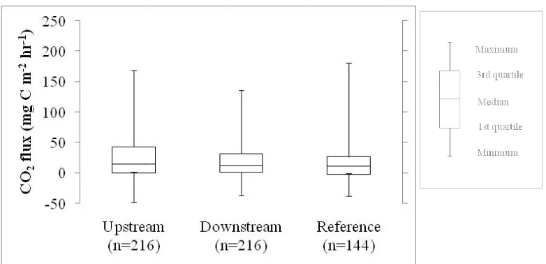
McBride 1994). ... 50 Fig. 2.7. Three-year period of measured CO2 flux in different sites. The number in
parentheses was the total samples collected in three years. The mean CO2 flux was the
lowest in the reference natural marsh (15.1 mg C m-2 hr-1), but the difference was only significant (P < 0.05) between the reference marsh the upstream marsh (26.5 mg C m-2 hr-1). ... 53 Fig. 2.8. Annual a) CO2 and b) CH4 fluxes in different years. Both CO2 and CH4 fluxes were
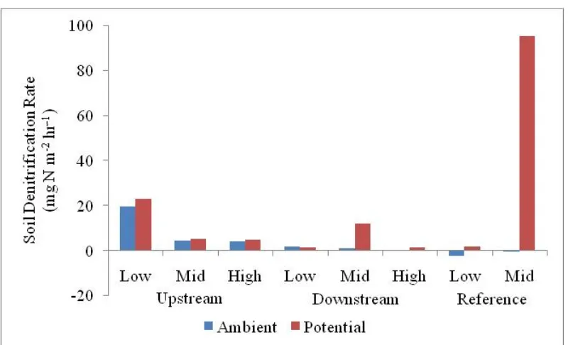
Fig. 2.10. Daily decomposition rates of the belowground plant tissues. Note: "Low", "Mid" and "High" represented the lowest, the middle and the highest elevations in each replicate block. ... 56 Fig. 2.11. The average ambient and potential soil denitrification rate in the brackish marsh. Note: "Low", "Mid" and "High" represented the lowest, the middle and the highest elevations in each replicate block. ... 58 Fig. 2.12. The soil CO2 fluxes in different vegetation zones measured during the study period
at the upstream in the created tidal marsh. The CO2 fluxes followed the pattern of the soil
temperature and they were significantly correlated (p < 0.001). The CO2 fluxes in the J.
roemerianus zone was slightly lower during many periods than the fluxes in other two
vegetation zones. ... 61 Fig. 2.13. The soil CH4 fluxes in different vegetation zones measured during the study period
at the upstream in the created tidal marsh. The CH4 fluxes followed the pattern of the soil
temperature although the correlation between them was insignificant. The lowest CH4 fluxes
were observed in the J. roemerianus zone. The magnitude of the CH4 flux was much smaller
than the observed soil CO2 flux. ... 61
Fig. 2.14. The redox potential at 30 cm depth in different vegetation zones in the upstream of the created tidal marsh between May 2012 and December 2013. The redox potential was the highest in the J. roemerianus dominated marsh (red line) where the ground elevation and the groundwater table depth was between that of S. alterniflora and the S. patens. ... 63 Fig. 3.1. The location of the research site (Phase II) in the North River Farms Restoration project (red). The site was a 14 ha brackish marsh created in 2007. ... 80 Fig. 3.2. The field installation of the infrared gas analyzer system (Li-8100A). ... 82 Fig. 3.3. The locations of the continuous CO2 flux measurement (green) and CO2 flux survey
in 2013. Note: elevation of surface water was referenced to the North American Vertical Datum of 1988 (NAVD88). Zero value for groundwater table depth on the y-axis indicates the soil surface. The grey area indicates the data missing periods that fitted from nearby dataloggers. ... 89 Fig. 3.5. The three day worth groundwater elevation (blue line) and surface water elevation (red line) data. The zero value at y-axis was the reference sea level elevation using North American Vertical Datum of 1988 (NAVD88). ... 90 Fig. 3.6. The monthly average CO2 flux and the relative average soil temperature. The CO2
flux showed a clockwise pattern and the flux was higher in the early year (March – June) than in the late year (July – November). ... 91 Fig. 3.7. the continuous CO2 flux (red) and the surface water elevation at the tidal stream
(blue) in (a) March; (b) May; (c) July; (d) November in 2013. The CO2 flux had more
intense changes during the tidal events at night except in August. ... 92 Fig. 3.8. The CO2 flux survey in (a) March and in (b) July. Note: The low, mid and high
marshes referred to the relative elevations at the sampling spots and the distance away from the tidal creek. Marsh 1 – downstream transect, Marsh 2 – upstream transect (See Fig. 3.3). ... 94 Fig. 3.9. The measured (blue) and the simulated CO2 flux (red) using the nested Q10 model
and groundwater table depth data (Eq. (6)) in (a) March; (b) May; (c) July; (d) November in 2013. The model underestimated the real flux and was not able to simulate the rapid flux variations due to the tidal fluctuation. ... 95 Fig. 3.10. The measured (blue) and the simulated CO2 flux (red) using the nested Q10 model
and surface water elevation data (Eq. (9)) in (a) March; (b) May; (c) July; (d) November in 2013. The model underestimated the real flux in the early year (March - June) and
overestimated the real flux in the late year (August – November). The model failed to
Fig. 3.11. The hourly averaged real CO2 flux (blue) and the simulated results (red) using the
nested Q10 model and surface water elevation data (Eq. (9)) in (a) March; (b) May; (c) July;
(d) November in 2013. The model failed to adequately simulate the real flux (R2 = 0.35). . 97 Fig. 3.12. The measured (blue) and the simulated CO2 flux (red) using the nested Q10 model
and surface water elevation data (Eq. (9)) in (a) March; (b) May; (c) July; (d) November in 2013. The data was separated to diurnal and nocturnal data based on the time of sunrise and sunset. The model failed to simulate the flux increasing due to the rising tides and the overall accuracy was lower than the results using the whole dataset. ... 99 Fig. 3.13. The measured (blue) and the simulated CO2 flux (red) using the nested Q10 model
and surface water elevation data (Eq. (9)) in (a) March; (b) May; (c) July; (d) November in 2013. The data was separated to March – June and July – November during simulations. The simulated flux was more close to the real flux than previous trials but failed to simulate the variation of the diel flux due to tides. ... 100 Fig. 3.14. The ideal flux rates using the nested Q10 model (Eq. (6)). The simulated flux was
positively correlated to the soil temperature, but negatively and positively correlated to the groundwater table depth when the soil temperature was > 20 °C and < 20 °C, respectively. ... 102 Fig. 3.15. The residual of the simulated flux from the nested Q10 model (Eq. (6)) in the (a)
early year (March – June) and (b) late year (July – November) in 2013. ... 104 Fig. 3.16. The measured (blue) and the simulated CO2 flux (red) using the tidally influenced
Q10 model (Eq. (11)) with WTD and T delays in (a) March; (b) May; (c) July; (d) November
in 2013. The data was separated to March – June and July – November during simulations. ... 107 Fig. 3.17. The simulated annual CO2 flux in the created brackish tidal marsh in 2013. The
highest CO2 flux was found in May and was the lowest in October and November. ... 110
Fig. 3.18. The simulated annual CO2 flux in the created brackish tidal marsh in 2012. The
highest CO2 flux was found in May and June and was the lowest in October and November.
Fig. 4.1. The relative location of the North River Farm created brackish tidal marsh
(highlighted in red). ... 127 Fig. 4.2. The relative locations of the GHG static chambers in the created marsh (orange squares) and in the natural marsh (green squares). ... 129 Fig. 4.3. The twelve transects of the plant harvesting experiments in March and August 2013. The tidal creek flows from left top toward the right bottom. The top 8 transects were in the created marsh and the 4 transects near the right bottom of the figure were located in the natural marsh (highlighted in green). ... 129 Fig. 4.4. The cross section view of two biomass harvesting transects. They were three sampling locations at each transect. The black arrows represent the relative sampling
elevation in the marsh along each transect. ... 130 Fig. C1. The targeted soil temperature datalogger (orange square) and the reference soil temperature datalogger (green square) used for gap fitting in the studied tidal brackish marsh. ... 200 Fig. C2. The linear regression of the soil temperature from the targeted soil temperature datalogger (y-axis) and the downstream low marsh datalogger (x-axis). ... 200 Fig. C3. The soil temperature at the upstream low marsh in 2013. The grey area indicates the data missing periods that fitted from the nearby datalogger. ... 201 Fig. C4. The targeted groundwater table depth datalogger (orange) and the reference
groundwater table depth dataloggers (green) used for gap fitting in the studied tidal brackish marsh. ... 202 Fig. C5. The linear regression of the groundwater table depth between the targeted datalogger (y-axis) and the two dataloggers (x-axis) at the a) right bank and b) left bank of the
Fig. C8. The linear regression of the surface water elevation between the targeted datalogger (y-axis) and the reference datalogger (x-axis) at the downstream. ... 204 Fig. C9. The surface water elevation at the upstream tidal creek in 2013. The grey area indicates the data missing periods that fitted from the nearby datalogger. ... 205 Fig. E1. The continuous monitoring of CO2 flux and the surface water elevation on March
5th 2013. ... 208 Fig. E2. The continuous monitoring of CO2 flux and the surface water elevation on April 3rd
2013. ... 209 Fig. E3. The continuous monitoring of CO2 flux and the surface water elevation on May 14th
2013. ... 209 Fig. E4. The continuous monitoring of CO2 flux and the surface water elevation on May 29th
2013. ... 210 Fig. E5. The continuous monitoring of CO2 flux and the surface water elevation on June 19th
2013. ... 210 Fig. E6. The continuous monitoring of CO2 flux and the surface water elevation on July 10th
2013. ... 211 Fig. E7. The continuous monitoring of CO2 flux and the surface water elevation on August
14th 2013. ... 211 Fig. E8. The continuous monitoring of CO2 flux and the surface water elevation on
September 18th 2013. ... 212 Fig. E9. The continuous monitoring of CO2 flux and the surface water elevation on
November 18th 2013. ... 212 Fig. F1. The observed and simulated CO2 fluxes and the groundwater table depth on March
5th 2013. ... 241 Fig. F2. The observed and simulated CO2 fluxes and the groundwater table depth on April
3rd 2013. ... 242 Fig. F3. The observed and simulated CO2 fluxes and the groundwater table depth on May
Fig. F4. The observed and simulated CO2 fluxes and the groundwater table depth on May
29th 2013. ... 243 Fig. F5. The observed and simulated CO2 fluxes and the groundwater table depth on June
19th 2013. ... 243 Fig. F6. The observed and simulated CO2 fluxes and the groundwater table depth on July
10th 2013. ... 244 Fig. F7. The observed and simulated CO2 fluxes and the groundwater table depth on August
14th 2013. ... 244 Fig. F8. The observed and simulated CO2 fluxes and the groundwater table depth on
September 18th 2013. ... 245 Fig. F9. The observed and simulated CO2 fluxes and the groundwater table depth on
CHAPTER 1: Introduction and Literature Review
Introduction
Greenhouse effect and global warming
The greenhouse effect is a process that occurs when solar radiation is reflected from the
Earth's surface and is transformed to heat by greenhouse gases warming the air temperature.
Major greenhouse gases (GHG) include water vapor, carbon dioxide (CO2), methane (CH4),
and nitrous oxide (N2O). Naturally produced greenhouse gases help keep the Earth's
temperature suitable for life, but human activities over the past 150 years increased the
concentrations of greenhouse gases in the atmosphere. Many believe this has intensified the
greenhouse effect, resulting in increased average air temperature, which has long range
climate implications.
From the 2007 Intergovernmental Panel on Climate Change (IPCC) report, the global
average CO2 concentration has increased from 280 ppm to 390 ppm in the past century.
Average global air temperature has increased 0.74 oC from 1900, and is forecasted to
increase 1.1 – 6.4 °C in the next hundred years in the continents of northern hemisphere. The
elevated temperature may bring problems such as sea level rise, change of ecosystems,
drought or flooding, and Antarctic sea ice melt (IPCC 2007).
Characteristics of greenhouse gases
Carbon dioxide is the major greenhouse gas in the atmosphere. Excess CO2 is mainly
emitted by human activities from industry, vehicles, and other combustion. There is 6 billion
(Miller 2001). The atmospheric lifetime of CO2 can be 50-200 years (IPCC 1996), and the
global average CO2 concentration reached 400 ppm in 2010 (IPCC 2014). The wavelengths
of infrared is between 0.7 – 1000 μm, and carbon dioxide absorbs wide infrared wavelengths
between 1 to 1000 μm, which is the main reason why CO2 is the most important greenhouse
gas. More than 80% of human produced CO2 emission is the combustion of fossil fuels from
electricity, transportation and industry (IPCC 2007). The main pathway of CO2 efflux in
nature is through respiration and it can be absorbed by plant uptake or dissolved in deep
oceans (Trenberth and Fasullo 2011).
Methane is the second most abundant greenhouse gas that contributes global warming.
Estimated global methane efflux is 310 million tons per year, and per emitted molecule, CH4
is 25 times more efficient than CO2 at trapping heat (IPCC 2007). The atmospheric life time
of CH4 is about 12 years (IPCC 1996) and methane receives and absorbs infrared
wavelengths between 3 to 9 μm. 60% of global methane emission come from human activity
and about 70% of the emission is from industry, agriculture and landfills (IPCC 2007). In
nature, it mainly emits from anaerobic soil, produced by methanogenic bacteria as anaerobic
decomposition occurs (Whiting and Chanton 2001).
Nitrous oxide is another important greenhouse gas that has ability to absorb infrared
energy with wavelengths between 2 to 9μm. Per emitted molecule, nitrous oxide is 298 times
more effective than carbon dioxide at trapping heat (IPCC 2007). The atmospheric life time
of N2O can be longer than 120 years, and it stimulates ozone depletion in the stratosphere
which comes from agriculture. Human produced N2O flux has been estimated to contribute
to 6% of global warming (IPCC 2007). In nature, nitrous oxide is a intermediate product in
Earth's nitrogen cycle, and it mainly releases when incomplete microbial denitrification
processes occur.
Wetlands and global warming
Wetlands are defined as inundated or saturated by surface or ground water at a
frequency and duration sufficient to support a prevalence of vegetation typically adapted for
life in saturated soil conditions (US Army Corps of Engineering). Wetlands provide variable
O2 conditions in both spatial and temporal scales among all types of ecosystems. Therefore,
wetlands have a potential to produce a wide range of greenhouse gases compared to other
ecosystems.
Ecological engineering technology is widely used for waste water treatment, habitat
restoration, ecosystem remediation, or storm water management. Wetlands are one type of
ecosystem that can be designed for these purposes. The net wetland loss was over 40 million
hectares in the U.S. since late 1970s, with a continued loss of 5,600 hectares per year from
2004 to 2009 (U.S. Fish and Wildlife Service). Wetland restoration aims to recover
ecosystem functions by recreating the hydrology and vegetation for a particular wetland type
(Zedler and Kercher 2005). Aquatic plants in wetlands absorb inorganic nutrients from
water, which can help remove excess nitrogen and phosphorus. Many wetland plants may
also actively transport oxygen from air into root zone and oxidize the rhizosphere, which
However, promoting nutrient removal from polluted water may also increase N2O emission
(Verhoeven et al. 2006). Moreover, because they are often anoxic, wetlands emit 15-40% of
total CH4 flux to the atmosphere (Bridgham 2006). Therefore, increasing wetland restoration
may potentially increase current greenhouse gas emissions.
Soil microbial respiration and GHG production
Greenhouse gas (GHG) emissions from nature are mainly due to complex soil
biogeochemical processes and can be affected by various environment factors. Most soil
microorganisms obtain energy from soil chemical oxidation-reduction (redox) reactions.
With oxidizing chemical substrates such as organic matter, sulfate, and dissolved carbon
dioxide from the soil pore water, soil microbes transform chemical compounds into different
intermediates and gain energy when electrons are transported from one substance to another.
The redox reactions of chemical compounds occur when net Gibb's free energy (ΔG) is less
than 0 so that the overall chemical reactions release energy to microorganisms. In a natural
ecosystem, chemical substrates such as oxygen, nitrate, manganese oxide, ferric iron, sulfate,
and carbon dioxide are the strong oxidizing agents that microbes can utilize without
providing extra energy. Greenhouse gases are often produced as the end products or
byproducts from soil microbial respiration.
Decomposition of organic matter (OM) involves various redox reactions. Electron flow
in the production of Adenosine Tri-Phosphate (ATP). During these redox reactions, CO2
releases as one of the oxidized products from organic matter.
In aerobic soil environments, oxygen (O2) serves as the electron acceptor and is reduced
to water (H2O) by microbes. When soil microbes are in an anaerobic environment, the
electron accepter is another chemical compound in soil that can replace O2. Soil microbes
utilize the chemical compounds in soil depending on their electron activity (EV). Common
chemical compounds involved in OM decomposition include nitrate (EV=0.749), manganese
dioxide (EV=0.526), ferric oxide (EV=-0.047), sulfate (EV=-0.222) and carbon dioxide
(EV=-0.244) (Schlesinger and Bernhardlt 2013).
When microbes reduce nitrate into nitrogen gas (i.e. denitrification), the intermediate
product N2O may directly release into atmosphere, creating a source for one of the major
greenhouse gases. The four steps of biochemical processes involved in denitrification
require four enzymes (Maier et al. 2000). One rate-limiting step in denitrification that affects
the presence of N2O is nitrous oxide reduction. The enzyme, nitrous oxide reductase, is acid
sensitive (i.e. is inhibited by low pH) and reacts with coenzymes such as sulfide, copper, and
nickel. The process also requires sufficient carbon sources, especially dissolved carbon, as
the electron provider. When nitrous oxide reduction is inhibited in the environment, N2O
accumulates and is released into the atmosphere (Coyne 1999).
Methanogenesis is another important biogeochemical process that produces methane as
an end product. There are two different microbial pathways that produce methane, both of
total methane produced in anaerobic environments is from acetate fermentation by
methanogens such as M. barkeri, M. mazei, and M. sohngenii (Gujer and Zehnder 1983;
Smith and Mah 1966; Schlesinger and Bernhardt 2013). Thirty percent of total methane is
from the redox reaction between hydrogen and CO2 and other smallcarbohydrates that
contain 1 – 2 carbon atoms by microorganisms (Thauer 1998; Maier et al. 2000; Schlesinger
and Bernhardt 2013) (Table 1.1). Methane can be oxidized into CO2 by methanotrophic
bacteria in soil (Coyne, 1999) or be photolyzed by sunlight in the troposphere (Fuglestvedt et
al. 1995).
Table 1.1. Different pathways of methanogenesis
Reaction ΔG°(kJ/mol)
- +
3 2 4
CH COO + H U CO + CH -36
2 2 4 2
4 H + CO UCH + 2 H O -131
- +
4 2 2
4HCOO + 4 H U CH + 3 CO + 2 H O -144.5
(modified from Thauer 1998)
Importance of sulfate in soil greenhouse gas emissions
Because sulfate has higher redox potential and releases more Gibb's free energy when
oxidizing soil organic matter than carbon dioxide, the presence of soil pore water sulfate in
estuarine wetlands may make the patterns in greenhouse gas emissions in these ecosystem
different than freshwater wetlands, especially in methane efflux. Concentration of soil pore
water sulfate affects the competition between sulfate reduction and fermentation of
Table 1.2). Wieder and Lang (1988) and Widdel (1988) measured the competition between
sulfate-reducing bacteria and methanogens in utilizing acetate and found sulfate-reducing
bacteria reduced acetate more efficiently than methanogens, leaving less available acetate in
soil pore space for methanogens. Some sulfate-reducing bacteria also use hydrogen as a
source of electrons and they are more efficient in utilizing hydrogen than methanogens
(Kristjansson et al. 1982). As a result, methanogenesis is inhibited in the environments with
high concentrations of soil pore water sulfate because energy sources (i.e. electron donors)
are mostly depleted when sulfate reduction occurs (Lovley and Phillips 1986; Kuivila et al.
1989).
In addition to methane emission, soil sulfate redox reactions may affect the dynamic of
carbon dioxide flux. Carbonic acid is the end product when sulfate-reducing bacteria
decompose organic compounds (Table 1.2). Since the total concentration of carbonic acids
in water is dependent on the partial pressure of carbon dioxide in the air (Henry's law) (
2 2 2 3
CO + H OU H CO ) with an equilibrium constant 1.7×10⁻³ at 25°C, the increased carbonic acid can vaporize from aqueous phase and release more CO2 into the atmosphere.
Weston et al. (2006) and Chambers et al. (2011, 2013) stated that the elevated sulfate
concentration stimulated the CO2 efflux because the present of sulfate in salt marsh soil
Table 1.2. Sulfate reducing reactions produce carbonic acids
Reaction ΔG°(kJ/mol)
- 2- - +
-3 4 3 3
2 CH CHOHCOO (lactate) + SO U 2 CH COO (acetate) + HS+ H + 2 HCO -160
- 2- +
-3 4 3
2 CH CHOHCOO + SO U 3 HS+ H + 6 HCO -255
- 2 - - +
-3 2 4 3 3
2 CH CH COO (propionate) + 3 SO U 4 CH COO + 3 HS+ H + 4 HCO -152
-
-3 3
2-4 CH COO 2 HCO
4Pyruvate+SO U 4 +H S+4 -356
-
-3 3
2- + -4
CH COO (acetate)+SO +3H U HS +2HCO -48
-3
2-2 4 HCO 2
4CH OH+3SO U 3HS−+4 +4H O+H+
-364 (Modified from Reddy and DeLaune 2008)
Some phototrophic sulfur oxidation bacteria, such as green (Chlorobium) and purple
sulfur bacteria (Rhodospirillum and Rhodopseudomonas), utilize sunlight as the energy
source and reduce CO2 to produce hydrocarbons (Reddy and DeLaune 2008). When this
reaction occurs in salt marshes, CO2 will be consumed by the microbes. Therefore, the CO2
flux in saline marshes may increase or remain similar to freshwater wetlands depended on
how the sulfate in soil and the activities of sulfate-reducing bacteria influence CO2 flux.
Nitrous oxide emission can also be affected by soil sulfate dynamics. Therefore,
oxidation of sulfur by one of the chemolithotrophic bacteria species, Thiobacillus, in
anaerobic environments has been shown to reduce NO3--N concentration in soil pore water,
resulting in less potential for mass loss of N2O (Coyne 1999).
The average molality of sulfate in seawater is 0.029 (Roy et al. 1993; Dickson 1990)
and salinity in water correlates to sulfate (SO42-) concentration. Brackish water marshes
contain a generally high percent of sulfate, which is the chemical need in microbial sulfate
In fresh water wetland ecosystems, N2O flux can range from -0.3 to 3.86 mg m-2 d-1
(Dinsmore et al. 2009; Hernandez and Mitsch 2006; Morse et al. 2012), CH4 flux may range
from -0.1 to 255.92 mg m-2 d-1 (Altor and Mitsch 2006; Dinsmore et al. 2009; Pulliam 1993; Waddington and Roulet 1996), and CO2 flux can range from -139 to 21,838 mg m-2 d-1
(Dinsmore et al. 2009; Morse et al. 2012; Stadmark and Leonardson 2005). However, in
brackish wetland ecosystems, the CH4 flux rate is negatively correlated to the salinity, as
shown by Bartlett et al. (1987), who found declining flux rates of 259 mg m-2 d-1 to 46.4 mg m-2 d-1 when the salinity increased from 0.4 to 26 ppt. The relation between CH4 flux and
salinity can be an overall log-linear relationship. The methane flux was found to be
negligible when sulfate concentration was more than 4mM by Poffenbarger et al. (2011).
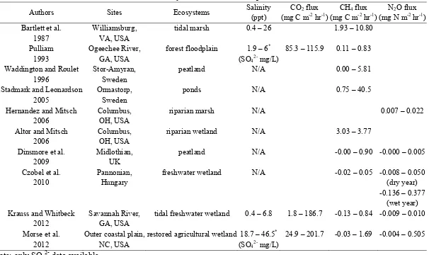
Table 1.3 summarizes the GHG fluxes and the associated salinity ranges measured in
previous research. Most of the previous research was conducted in freshwater ecosystems or
coastal wetlands with low salinity. Not many studies that have been conducted in tidal
brackish marshes and even fewer studies have been studied on created tidal marshes to
Table 1.3. Summary of the GHG fluxes in previous research
Authors Sites Ecosystems Salinity (ppt)
CO2 flux (mg C m-2 hr-1)
CH4 flux (mg C m-2 hr-1)
N2O flux (mg N m-2 hr-1) Bartlett et al.
1987
Williamsburg, VA, USA
tidal marsh 0.4 – 26 1.93 – 10.80
Pulliam 1993
Ogeechee River, GA, USA
forest floodplain 1.9 – 6* (SO42- mg/L)
85.3 – 115.9 0.11 – 0.83
Waddington and Roulet 1996
Stor-Amyran, Sweden
peatland N/A 0.00 – 5.81
Stadmark and Leonardson 2005
Ormastorp, Sweden
ponds N/A 0.75 – 40.5
Hernandez and Mitsch 2006
Columbus, OH, USA
riparian marsh N/A 0.007 – 0.022
Altor and Mitsch 2006
Columbus, OH, USA
riparian wetland N/A 3.03 – 3.77
Dinsmore et al. 2009
Midlothian, UK
peatland N/A -0.00 – 0.90 -0.000 – 0.005
Czobel et al. 2010
Pannonian, Hungary
freshwater wetland N/A -0.02 – 0.05 -0.008 – 0.050 (dry year) -0.136 – 0.377
(wet year) Krauss and Whitbeck
2012
Savannah River, GA, USA
tidal freshwater wetland 0.4 – 6.8 1.8 – 186.7 -0.13 – 0.84 -0.009 – 0.010
Morse et al. 2012
Outer coastal plain, NC, USA
restored agricultural wetland 18.7 – 46.5* (SO42- mg/L)
24.9 – 201.7 -0.03 – 1.69 -0.004 – 0.505
*Note: only SO
Other potential environmental factors that influence GHG emissions
Beside concentration of pore water sulfate, several other environment factors such as
plant types, hydroperiod and precipitation can affect biogeochemical processes and GHG
fluxes in wetlands.
Plant biomass has different characteristics and structures that can have various
decomposition rates when they are utilized by microbes as the electron donor. Some
components like cellulose can be decomposed first while lignin usually remains decades
before being decomposed (Coyne 1999). Wynn and Bird (2007) determined the
decomposition rate of the soil organic matter that was produced by C3 and C4 plants. Their
result showed the soil organic carbon (SOC) from C4 plants was decomposed faster than the
SOC from C3 plants. The decomposition rate was 45% for Spartina alterniflora (C4 plant)
in a 60-day experiment (Yang et al. 2009).
Precipitation and groundwater table proximity to the soil surface directly affects aerobic
and anaerobic respiration occurring in wetland soils. A larger anaerobic area and longer
inundation period increases the potential for denitrification and methanogenesis to occur
because microorganisms must use an electron accepter other than O2. Basically, the soil
respiration rate positively correlates to temperature and after precipitation because of the
rising soil moisture availability (Raich and Schlesinger 1992). Czobel et al. (2010) measured
the N2O and CH4 fluxes in different wetlands, and compared them with the soil moisture.
fluxes were -0.008 to 0.05 mg N m-2 day-1 in the dry year and -0.136 to 0.377 mg N m-2 day-1 in the wet year in Sárospatak, Hungary.
Krauss and Whitbeck (2012) measured the greenhouse gas fluxes from three replicates
in a tidal fresh water wetland in South Carolina and Georgia. Over a two-year period study,
they found the CO2 flux ranged from 6.7 to 684.5 mg CO2 m-2 hr-1, CH4 flux was -0.17 to
1.12 mg CH4 m-2 hr-1 and N2O flux was -0.035 to 0.031 mg N2O m-2 hr-1. The CO2 flux was
significant to the time, water level, and soil temperature. The CO2 flux increased when the
soil temperate rose or when water level dropped, while the CH4 flux only correlated to
sampling time. The N2O flux had no correlation to any environment factors in this study.
Besides the environmental factors affecting long term GHG emissions, some rapidly
changing factors such as the groundwater table in tidal marsh ecosystems may alter the GHG
fluxes on a daily basis. Some research had been conducted using different methods to
measure short term GHG flux rates. Yamamoto et al. (2009) used the static chamber method
to measure the daily changes of CO2 and CH4 fluxes within a tidally influenced brackish bay
(Lake Obuchi) in Japan. They found the GHG flux rates were positively correlated with
water table elevation (p < 0.001) during spring tides. When the tide pushed water into the
marsh, the CO2 flux rates increased from 400 to 750 mg CO2 m-2 hr-1 while CH4 flux rates
increased from 10 to 40 mg CH4 m-2 hr-1. The flux rates decreased to initial rates after the
tide dropped in 2 of the 3 vegetation zones closest to the bay.
Kathilankal et al. (2008) used an eddy-flux infrared gas analyzer to measure the CO2
could change CO2 flux by 0.83 g CO2 m-2 d-1. They stated the soil and plant respiration could
be inhibited when the soil was inundated, and the sunlight intensity could alter the CO2
assimilation rate of plants from 1 g CO2 m-2 d-1 on sunny days to 0.41 g CO2 m-2 d-1 on
cloudy days.
McDermitt et al. (2011) measured the methane flux in Florida everglades by using an
eddy-flux near-infrared laser gas analyzer and found the CH4 flux rate was higher during the
day than at night. A similar conclusion was stated by Detto et al. (2011). They measured
both the CH4 and CO2 emissions continuously in a restored emergent wetland in
Sacramento-San Joaquin, Delta, California, and found the emissions of CH4 and CO2 changed across the
day.
Methods of soil greenhouse gas sampling
Several sampling methods that have been widely used in measuring
biosphere-atmosphere exchange of greenhouse gases in the field. The most common method for trace
gas sampling is using a chamber technique which encloses a volume of air on top of the soil
surface to capture emitted gas (Mosier 1990; Lapitan et al. 1999). Two versions of basic
chamber designs have been used to estimate fluxes of CO2, CH4, N2O, NO, and H2S since the
1970s (Kucera and Kirkham 1971; Kanemasu et al. 1974; Bartlett et al. 1987; Pulliam 1993;
Magenheimer et al. 1996; Neubauer et al. 2000; Ford et al. 2012; Krauss and Whitbeck
2012).
A static (closed-top) chamber is designed to restrict gas exchanges between the inside
concentrations of the gases build up inside the chamber during the sampling period, and this
method may under estimate gas fluxes due to lack of air turbulence that should normally
occur (Jury et al. 1982; Mosier 1990). A dynamic (open-top) chamber is designed to
eliminate the errors that a closed chamber method may have. It is coupled with an inlet and
an outlet for air flows through the chamber, and the samples are collected at both ends of the
chamber to allow for calculation of the difference of gas concentrations. However, trace
gases such as CH4 and N2O fluxes may be difficult to measure using a dynamic chamber
compared to a static chamber because the concentrations may under detection limits (Crill
1991;Hutchinson and Mosier 1981). Conen and Smith (1998) re-examined different
chamber methods for measuring trace gas fluxes, and found the static (closed-top) chamber
technique was the best method in field trace gas sampling.
The collected samples from the chamber techniques are analyzed using gas
chromatography in laboratories or using in-situ non-dispersive infrared gas analysis. Gas
chromatography has been the most widely used analytical method for CO2, CH4 and N2O
fluxes (Lucera and Kirkham 1971; Kanemasu et al. 1974; Pulliam 1993;Magenheimer et al.
1996; Ford et al. 2012; Krauss and Whitbeck 2012). However, more research has used
infrared gas analysis to capture the flux changes in recent years (Xu and Qi 2001; Vargas and
Allen 2008; Savage et al. 2009; Jia et al. 2013; Miao et al. 2013; Han et al. 2014) because it
provides results of trace gas concentrations in much shorter periods (1/20 – 1 second) and
Another widely used measuring method in the field is the eddy correlation technique. It
detects concentrations of trace gases with an infrared gas analyzer at a certain height above
the soil surface and correlates the concentrations with vertical wind velocity using
aerodynamic models. It can measure trace gas fluxes from a process level, ecosystem level,
or regional level. It has been used to measure continuous gas fluxes in different ecosystems
(Wang et al. 2009;McDermitt et al. 2011). However, the technique is complicated to operate
and errors can occur due to signal noises, instrument drift, inaccurate vertical alignment, and
inadequate sampling height (Businger 1986).
Several other sampling methods such as static alkali absorption method (Jensen et al.
1996; Yim et al. 2002) and gradient method (Tang et al. 2003; Flechard et al. 2007; Maier
and Schack-Kirchner 2014) have also been used for estimating biosphere-atmosphere
exchange of greenhouse gases.
Importance of blue carbon to climate change
Blue carbon is the carbon that is stored in living organisms and soil sediments in oceans
and coastal ecosystems such as tidal marshes, mangroves, and seagrass beds. Oceans are the
largest carbon sink on Earth, and store more than a total of 3.8 Pg (billion tons) of carbon.
Coastal ecosystems sequester CO2 from the atmosphere through plant primary production
and is stored in soil sediments. Research has estimated overall carbon sequestration rates of
carbon at a rate up to 100 times faster than terrestrial forest ecosystems (Kennedy and Bjork
2009; Chmura et al. 2003; Pidgeon 2009) (Table 1.4).
Since carbon sequestration is so high in tidal marshes, restoration of these areas could
be an important method to sequester carbon. In an analysis by Craft et al. (1999), salt marsh
accumulation rates of soil organic carbon and total nitrogen in the constructed marshes
decreased with age. The highest accumulation rates were 99 g m-2 yr-1 for organic carbon (OC) and 12.5 g m-2 yr-1 for total nitrogen (TN) in one-year old wetlands, while the
accumulation rates of OC and TN decreased to 39 g m-2 yr-1 and 2.6 g m-2 yr-1 in a 28-year old wetland (Craft et al. 2003). Restored marshes and natural marshes could have similar
aboveground biomass, but in a study by Krull and Craft (2009), the accumulation rates of OC
(260 ± 40 g m-2 yr-1) and TN (11 ± 3 g m-2 yr-1) in the soil were higher in the restored marshes than the natural marshes. Carbon sequestration rates may not be different in saline
marshes despite their climate regime (Chmura et al. 2003). Different plant species may also
contain different capacity of carbon pools. Elsey-Quirk et al. (2011) found the average plant
Table 1.4. Carbon storage rate and carbon stock in different ecosystems
Ecosystem type
Carbon stock (g C m-2)
Carbon storage rate (g C m-2 yr-1)
Total global area (×1012 m2)
Total potential C storage (tons CO2 per year)
Plants Soil
Tidal marshes Unclear 210 0.22 169,400,000
Seagrass 184 7000 83 0.152 46,258,667
Mangroves 7990 139 0.3 152,900,000
Tropical forests 12045 12273 2.4 22.5 198,000,000
Temperate forests 5673 9615 6.7 10.4 255,493,333
Boreal forests 6423 34380 1.5 13.7 75,350,000
(Modified from Pidgeon 2009). Multiply 3.67 to convert the unit to g CO2 m-2 yr-1.
However, 25 – 50% of vegetated coastal ecosystems were lost over the last hundred
years due to human activity and climate change, and 30 – 40% of coastal ecosystems could
be lost in the next century (Mcleod et al. 2011; Pendleton et al. 2012). When these coastal
ecosystems are degraded, the soil carbon may be decomposed through soil microbial activity
and release as greenhouse gas to the air (Pendleton et al. 2012).
In order to achieve the reduction of global GHG emissions, 40 national and 20
sub-national jurisdictions initiated charges on carbon emission by either adding carbon tax or
established carbon cap and trade system to reduce 6 GtCO2e of the annual global GHG
emissions (World Bank 2014).
Despite various critiques about these two programs, the carbon cap and trade was
considered to be a more practical method and have been initially successful in the European
Union Emissions Trading Scheme (EU ETS) (Ellerman and Buchner 2007; Stavins 2008).
The unit price range of per tonne of CO2 was widely varied between 1 (Bew Zealand CaT) –
Cap and Trade Program (California CaT), and the price per tonne of CO2e emission was
around 11 – 12 dollars in 2014, which was at the lower end of the global price range.
Although the area of global tidal marshes account for less than 1% of the total area of
the ecosystems listed on Table 1.4, tidal marshes contribute about 15% of the global carbon
sequestration and generate a potential of 13.3 billion dollars of carbon credits each year.
The carbon sequestration and greenhouse gas emissions from brackish salt marshes has
been studied very little, with none of the research focused on restored brackish tidal marshes.
The daily changes of the GHG fluxes also need to be studied since the fast changes of
environmental conditions in tidal marsh systems may create large daily variation of GHG
fluxes. In addition, net carbon sequestration from the atmosphere is expected to occur in
nature because of the high primary production but the theory is yet to be quantified.
With higher salinity and more frequent tidal flushing that brackish tidal marshes
provide, they can be ideal systems for carbon sequestration as well as provide ecosystem
services and water quality improvement. Fluctuation of tides results in frequent change of
environment variables make the system complex but worthwhile to study.
Research objectives
The primary goal of this research was to determine the relationship of GHG fluxes to
environmental variables and evaluate whether a created brackish salt marsh can be an
effective carbon sink. To evaluate the effective GHG emissions from the created brackish
three year period between March 2011 – November 2013. To quantify the carbon
sequestration rate in the created brackish marsh, a mass balance was calculated by measuring
both carbon output (CO2 and CH4 efflux) and carbon input (plant primary production) to the
marsh during the growing season of 2013. Specific objectives for this research include:
1. Determining GHG fluxes and the relationship among environment variables in the
created brackish wetland (salinity>20) on a long term (monthly) and short term (daily)
basis. (Chapters 2 and 3)
2. Improve long term predictions of the GHG fluxes. (Chapter 3)
3. Evaluating the carbon sequestration efficiency of the created brackish wetland.
(Chapter 4)
References
Altor, A. E., & Mitsch, W. J. (2006). Methane flux from created riparian marshes:
Relationship to intermittent versus continuous inundation and emergent
macrophytes. Ecological Engineering, 28, 224-234.
Bartlett, K. B., Bartlett, D. S., Harriss, R. C., & Sebacher, D. I. (1987). Methane
emissions along a salt-marsh salinity gradient. Biogeochemistry, 4(3),183-202.
Bridgham, S. D., Megonigal, J. P., Keller, J. K., Bliss, N. B., & Trettin, C. (2006). The
carbon balance of North American wetlands. Wetlands, 26, 889-916.
Brix, H. (1997). Do macrophytes play a role in constructed wetlands? Water Science
Businger, J. A. (1986). Evaluating the accuracy with which dry deposition can be
measured with current micrometeorological techniques. Journal Climate and
Applied Meteorology, 25, 1100-1124.
Chambers, L. G., Reddy, K. R., & Osborne, T. Z. (2011). Shortterm response of carbon
cycling to salinity pulses in a freshwater wetland. Soil Science Society of America
Journal, 75, 2000–2007.
Chambers, L. G., Osborne, T. Z., & Reddy, K. R. (2013). Effect of salinity pulsing events on
soil organic carbon loss across an intertidal wetland gradient: a laboratory
experiment. Biogeochemistry, 115, 363–383.
Chmura, G. L., Anisfeld, S. C., Cahoon, D. R., & Lynch, J. C. (2003). Global carbon
sequestration in tidal, saline wetland soils. Global Biogeochemical Cycles,
17(4), 22-1-22-12.
Conen, F. & Smith, K. A. (1998). A re-examination of closed flux chamber methods for
the measurement of trace gas emissions from soils to the atmosphere. European
Journal of Soil Science, 49, 701-707.
Coyne, M. (1999). Soil Microbiology: An Exploratory Approach. New York, USA:
Delmar Publishers.
Craft, C., Reader, J., Sacco, J. N., & Broome, S. W. (1999). Twenty-five years of
ecosystem development of constructed Spartina alterniflora (loisel) marshes.
Ecological Applications, 9(4), 1405-1419.
Sacco, J. (2003). The pace of ecosystem development of constructed Spartina
alterniflora marshes. Ecological Applications, 13(5), 1417-1432.
Crill, P. M. (1991). Seasonal patterns of methane uptake and carbon dioxide release by a
temperate woodland soil. Global Biogeochemical Cycle, 5, 319-334.
Czobel, S., Horvath, L., Szirmai, O., Balogh, J., Pinter, K., & Nemeth, Z. (2010).
Comparison of N2O and CH4 fluxes from pannonian natural ecosystems.
European Journal of Soil Science, 61(5), 671-682. doi:10.1111/j.1365-2389.2010.01275.x ER
Detto, M., Verfaillie, J., Anderson, F., Xu, L., & Baldocchi, D. (2011). Comparing
laser-based open- and closed-path gas analyzers to measure methane fluxes using the
eddy covariance method. Agricultural and Forest Meteorology, 151,
1312-1324.
Dickson, A. G. (1990). Standard potential of the reaction:
AgCl(s)+1/2H2(g)=Ag(s)+HCl(aq), and the standard acidity constant of the ion
HSO4- in synthetic sea water from 273.15 to 318.15 K. Journal of Chemical
Thermodynamics, 22, 113-127.
Dinsmore, K. J., Skiba, U. M., Billett, M. F., Rees, R. M., & Drewer, J. (2009). Spatial
and temporal variability in CH4 and N2O fluxes from a Scottish ombrotrophic
peatland: Implications for modelling and up-scaling. Soil Biology and
Biochemistry, 41, 1315-1323.
on the oceanic carbon cycle. Biogeosciences, 2, 1-8.
Ellerman, D. & Buchner, B. (2007). The European Union emissions trading scheme:
origins, allocation, and early results. Review of Environmental Economics and
Policy, 1, 66-87.
Elsey-Quirk, T., Seliskar, D. M., Sommerfield, C. K., & Gallagher, J. L. (2011). Salt
marsh carbon pool distribution in a mid-Atlantic lagoon, USA: sea level rise
implications. Wetlands, 31(1), 87-99.
Flechard, C., Neftel, A., Jocher, M., Ammann, C., Leifeld, J. & Fuhrer, J. (2007).
Temporal changes in soil pore space CO2 concentration and storage under
permanent grassland. Agricultural and Forest Meteorology, 142 (1), 66–84.
Ford, H., Garbutt, A., Jones, L. & Jones, D. L. (2012). Methane, carbon dioxide and
nitrous oxide fluxes from a temperate salt marsh: Grazing management does
not alter global warming potential. Estuarine, Coastal and Shelf Science, 113,
182-191.
Forster, P., Ramaswamy, V., Artaxo, P., Berntsen, T., Betts, R., Fahey, D.W., Haywood,
J., Lean, J., Lowe, D.C., Myhre, G., Nganga, J., Prinn, R., Raga, G., Schulz,
M., & Dorland, R. V. (2007). Changes in Atmospheric Constituents and in
Radiative Forcing. In: Climate Change 2007: The Physical Science Basis. Contribution of Working Group I to the Fourth Assessment Report of the Intergovernmental Panel on Climate Change [Solomon, S., D. Qin, M.
Cambridge, United Kingdom and New York, NY, USA: Cambridge University
Press.
Fuglestvedt, J. S., Jonson, J. E., Wang, W. C., & Isaksen, I. S. A. (1995). Responses in
tropospheric chemistry to changes in UV fluxes, temperatures and water vapour
densities. NATO Advanced Science Institutes, 32, 145-162.
Han, G., Luo, Y., Li, D., Xia, J., Xing, Q. & Yu, J. (2014). Ecosystem photosynthesis
regulates soil respiration on a diurnal scale with a short-term time lag in a
coastal wetland. Soil Biology and Biochemistry, 68, 85-94.
Hernandez, M. E., & Mitsch, W. J. (2006). Influence of hydrologic pulses, flooding
frequency, and vegetation on nitrous oxide emissions from created riparian
marshes. Wetlands, 26, 862-877.
Hutchinson, G. L. and Mosier, A. R. (1981). Improved soil cover method for field
measurement of nitrous oxide fluxes. Soil Society of American Journal, 45,
311-316.
Gujer, W. & Zehnder, A. J. (1983). Conversion processes in anaerobic digestion. Water
Science and Technology, 15, 49-77.
IPCC (1996). Technical Paper IV: Implications of Proposed CO2 Emissions Limitations.
Retrieved from IPCC website:
http://www.ipcc.ch/pdf/technical-papers/paper-IV-en.pdf
IPCC. (2007). Climate Change 2007: Synthesis Report. Retrieved from IPCC website:
Jensen, L.S., Mueller, T., Tate, K.R., Ross, D.J., Magid, J. & Nielsen, N.E. (1996). Soil
surface CO2 flux as an index of soil respiration in situ: a comparison of two
chamber methods. Soil Biology and Biochemistry, 28, 1297–1306.
Jia, X., Zha, T., Wu., B., Zhang, Y., Chen, W., Wang, X., Yu, H. & He, G. (2013).
Temperature response of soil respiration in a Chinese pine plantation:
hysteresis and seasonal vs. diel Q10. PLOS ONE, 8(2), e57858.
Jury, W. A., Letey, L. & Collins, T. (1982). Analysis of chamber methods used for
measuring nitrous oxide production in the field. Soil Society of America, 46,
250-256.
Kanemasu, E. T., Powers, W. L. & Sij, J. W. (1974). Field chamber measurements of
CO2 flux from soil surface. Soil Science, 118(4), 233-237.
Kathilankal, J. C., Mozdzer, T. J., Fuentes, J. D., D'Odorico, P., McGlathery, K. J., &
Zieman, J. C. (2008). Tidal influences on carbon assimilation by a salt marsh.
Environmental Research Letters, 3(4), 1-6.
Kennedy, H. & Bjork, M. (2009). Seagrass Meadows. The management of natural
coastal carbon sinks, IUCN, 23-30.
Krauss, K. W., & Whitbeck, J. L. (2012). Soil greenhouse gas fluxes during wetland
forest reteat along the lower Savannah River, Georgia (USA). Wetlands, 32,
73-81.
Kristjansson, J. K., Schonheit, P. & Thauer, R. K. (1982). Different Ks-values for
explanation for the apparent inhibition of methanogenesis by sulfate. Archives
of Microbiology, 131, 278–282.
Krull, K., & Craft, C. (2009). Ecosystem development of a sandbar emergent tidal marsh,
Altamaha River estuary, Georgia, USA. Wetlands, 29(1), 314-322.
Kucera, C. L. & Kirkham, D. R. (1971). Soil respiration studies in tallgrass prairie in
Missouri. Ecology, 52(5), 912-915.
Kuivila, K. M., Murray, J. W., Devol, A. H. & Novelli, P. C. (1989). Methane
production, sulfate reduction and competition for substrates in the sediments of
Lake Washington. Geochimica et Cosmochimica Acta, 53, 409–416.
Lapitan, R. L., Wanninkhof, R. & Mosier, A. R. (1999). Methods for stable gas flux
determination in aquatic and terrestrial systems. Approaches to Scaling a
Trace Gas Fluxes in Ecosystems, 29-66.
Lovley, D. R. & Phillips, E. J. P. (1986). Organic matter mineralization with reduction of
ferric iron in anaerobic sediments. Applied and Environmental Microbiology,
51, 683–689.
Magenheimer, J. F., More, T. R., Chmura, G. L. & Daoust, R. J. (1996). Methane and
carbon dioxide flux from a macrotidal salt marsh, bay of Fundy, New
Brunswick., Estuaries, 19(1), 139-145.
Maier, M. & Schack-Kirchner, H. (2014). Using the gradient method to determine soil
Maier, R. M., Pepper, I. L., & Gerba, C. P. (2000). Environmental Microbiology.
California, USA: Academic Press.
McDermitt, D., Burba, G., Xu, L., Anderson, T., Komissarov, A., Riensche, B.,
Schedlbauer, J., Starr, G., Zona, D., Oechel, W., Oberbauer, S., & Hastings, S.
(2011). A new low-power, open-path instrument for measuring methane flux by
eddy covariance. Applied Physics B, 102, 391-405.
Mcleod, E., Chmura, G. L., Bouillon, S., Salm, R., Bjork, M., Duarte, C. M., Lovelock,
C. E., Schlesinger, W. H. & Silliman, B. R. (2011). A blueprint for blue carbon:
toward an improved understanding of the role of vegetated coastal habitats in
sequestering CO2. The ecological Society of America, 9(10), 552-560.
Miao, G., Noormets, A., Domec, J., Trettin, C. C., McNulty, S. G., Sun, G. & King, J. S.
(2013). The effect of water table fluctuation on soil respiration in a lower
coastal plain forested wetland in the southeastern U.S.. Journal of Geophysical
Research: Biogeosciences, 118, 1748-1762.
Miller, G. T. Jr. (2001). Living in the Environment. California, USA: Wadsworth
Publishing Co.
Morse, J. L., Ardon, M., & Bernhardt, E. S. (2012). Greenhouse gas fluxes in
southeastern U.S. coastal plain wetlands under contrasting land uses.
Ecological Applications, 22(1), 264-280.
Mosier, A. R. (1990). Gas flux measurement techniques with special reference to
Soil and the Greenhouse Effect, 289-301.
Neubauer, S. C., Miller, W. D. & Anderson, I. C. (2000). Carbon cycling in a tidal
freshwater marsh ecosystem: a carbon gas flux study. Marine Ecology
Progress Series, 199, 13-30.
Pendleton, L., Donato, D. C., Murray, B. C., Crooks, S., Jenkins, W. A., Sifleet, S., Craft,
C., Fourqurean, J. W., Kauffman, J. B., Marba, N., Megonigal, P., Pidgeon, E.,
Herr, D., Gordon, D. & Baldera, A. (2012). Estimation global "Blue Carbon"
emissions from conversion and degradation of vegetated coastal ecosystems.
PLOS ONE, 7(9), 1-7.
Pidgeon, E. (2009). Carbon sequestration by coastal marine habitats: important missing
sinks. The management of natural coastal carbon sinks, IUCN, 47-51.
Poffenbarger, H. J., Needelman, B. A., & Megonigal, J. P. (2011). Salinity influence on
methane emissions from tidal marshes. Wetlands, 31(5), 831-842.
Pulliam, W. M. (1993). Carbon dioxide and methane exports from a southeastern
floodplain swamp. Ecological Monographs, 63, 29-53.
Raich, J. W., & Schlesinger, W. H. (1992). The global carbon-dioxide flux in soil
respiration and its relationship to vegetation and climate. Tellus Series
B-Chemical and Physical Meteorology, 44(2), 81-99.
Reddy, K. R. & DeLaune, R. D. (2008). Biogeochemistry of Wetlands: Science and
Applications. New York, USA: CNC Press.