Inventory Optimization in a One Product Recoverable Manufacturing System

ABSTRACT

AHISKA, SEMRA SEBNEM. Inventory Optimization in a One Product Recoverable Manufacturing System. (Under the direction of Dr. Russell E. King and Dr. Thom J. Hodgson.)

Environmental regulations or the necessity for a “green image” due to growing

environmental concerns as well as the potential economical benefits of product recovery have pushed manufacturers to integrate product recovery management with their

manufacturing process. Consequently, production planning and inventory control of recoverable manufacturing systems has gained significant interest among researchers who aim to contribute to industrial practice. This dissertation considers inventory optimization of a single product recoverable manufacturing system where stochastic demand is met by either newly manufactured items or remanufactured items. Lead times and set up costs for manufacturing and remanufacturing are considered. The inventory optimization problem for this system is formulated as a Markov decision process (MDP) and through an empirical study, optimal or near-optimal policy characterizations under several cost configurations and several lead time cases for manufacturing and

remanufacturing are determined. The effects of a change in cost parameters of the system on the optimal policy structure as well as policy parameter values are

Inventory Optimization in a One Product Recoverable Manufacturing System

by

Semra Sebnem Ahiska

A dissertation submitted to the Graduate Faculty of North Carolina State University

in partial fulfillment of the requirements for the Degree of

Doctor of Philosophy

Industrial and Systems Engineering

Raleigh, North Carolina

2008

APPROVED BY:

Dr. Russell E. King Dr. Thom J. Hodgson

Chair of Advisory Committee Co-chair of Advisory Committee

DEDICATION

To my parents and my aunts, who have always encouraged me to complete my studies no matter

BIOGRAPHY

S. Sebnem Ahiska was born in Istanbul, Turkey on January 30, 1978. For her secondary education, she attended Sainte Pulchérie French middle school and Saint Joseph French High school. She received her Bachelor of Science in Industrial Engineering from Istanbul Technical University in 2001. Upon graduation, she attended Galatasaray

University where she received her Master’s degree in Industrial Engineering in 2003. She received a scholarship from the Council of Higher Education of Turkey for her PhD education in USA, and she began her PhD education in Industrial and Systems

Engineering at North Carolina State University in 2004. Her research interests include the applications of Operations Research, Markov Decision Processes, mathematical

ACKNOWLEDGMENTS

I would like to especially thank Dr. Russell E. King for all his help, support, guidance, and valuable advices he has given me during my PhD education. I would also like to thank Dr. Thom Hodgson, Dr. Kristin Thoney and Dr. Jeffrey Joines for their valuable comments regarding my dissertation.

TABLE OF CONTENTS

List of Tables……….vii

List of Figures………xii

1. Introduction………..… …1

2. Literature survey on inventory control in recoverable manufacturing systems………. 5

2.1. Deterministic recoverable inventory models………... 6

2.2. Stochastic recoverable inventory models……….. 8

2.2.1. Periodic-review models………. 9

2.2.2. Continuous-review models……….. 10

3. Inventory optimization for a periodically-reviewed recoverable manufacturing system……….. 15

3.1. Problem description and MDP formulations ………... 18

3.2. Experiments setting and the analysis………....……….. 24

3.3. Results regarding policy structures under different lead time cases……….. 26

3.3.1. Results for unity lead time case for both manufacturing and remanufacturing………. 26

3.3.2. Results for the case where remanufacturing lead time is two periods and manufacturing lead time is one period…... 34

3.3.3. Results for the case where remanufacturing lead time is one period and manufacturing lead time is two periods ……… 36

3.4. Sensitivity analysis regarding the effect of changing the coefficient of variation of demand distribution on the optimal policy……… 38

3.5. Discussion….……….. 41

4. Inventory policy characterization methods for a single-product recoverable system… 43 4.1. The recoverable system………... 44

4.2. An MDP-based search methodology and a factorial analysis……… 45

4.3. A neural network analysis………... 53

5. Inventory policy characterizations for a single-product recoverable system over

different stages of the product life cycle……….. 58

5.1. Problem description……… 59

5.2. Product life cycle analysis………. 60

5.3. Results………. 64

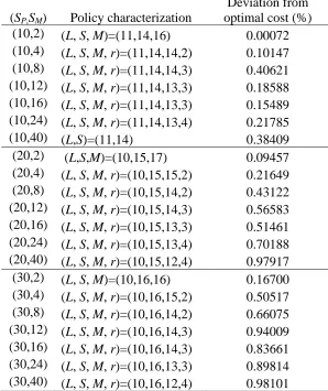
5.3.1. The policy characterizations over different stages of product life cycle under different set up cost configurations……… 65

5.3.2. The performance comparison of the PULL policy with the MDP-based policy characterizations………... 71

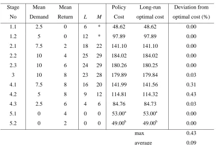
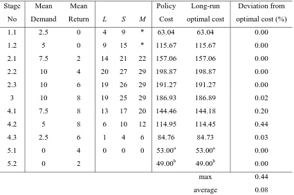
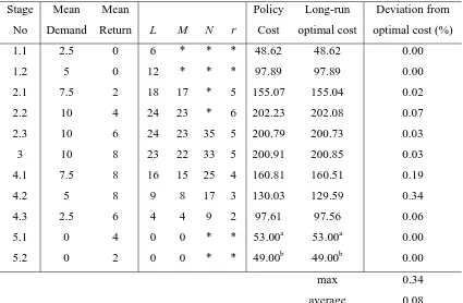
5.3.3. The performance evaluation of long run optimal or near-optimal policy characterizations in a finite horizon setting……… 75

5.3.4. Frequent policy revision vs. no revision or partial revision in finite-horizon setting………... 76

5.4. Discussion.……….. 78

6. Conclusion and further work………. 79

References……….. 82

LIST OF TABLES

Table 3.1 The cost parameters and the corresponding values considered in the experiments……… 26 Table 3.2 The effect of changing holding cost for serviceable items, CHS, when

lp=lm=1………28 Table 3.3 The effect of changing holding cost for recoverable items, CHR, when

lp=lm=1………29 Table 3.4 The effect of changing backordering cost, CBO, when lp=lm=1………….. 29

Table 3.5 The effect of changing disposal cost for recoverable items, CDISP, when lp=lm=1………29 Table 3.6 The effect of changing lost sales cost, CLS, when lp=lm=1………. 30 Table 3.7 The effect of changing set up cost for regular production, SP, when

lp=lm=1………...30 Table 3.8 The effect of changing set up cost for remanufacturing, SM, when

lp=lm=1………....31 Table 3.9 Results in the existence of non-zero manufacturing and remanufacturing

set up costs, SP and SM, when lp=lm=1……… 33 Table 3.10 The summary of policy structures found in the experiments for case lp=1

& lm=2……… 36 Table 3.11 The summary of policy structures found in the experiments for case lp=2

& lm=1……… 37 Table 3.12 Summary of the results of experiments on CV of demand distribution… 40 Table 4.1 Relevant cost parameters and their respective values considered in the

factorial analysis……… 46 Table 4.2 System parameters that are kept unchanged during the factorial

analysis………... 47 Table 4.3 Appropriate policy structures with respect to set up cost structure of the

Table 4.4 Factorial analysis results for lead time case 1: lp=lm=1………. 51 Table 4.5 Factorial analysis results for lead time case 2: lp=2; lm=1………. 52 Table 4.6 Factorial analysis results for lead time case 3: lp=1; lm=2………. 52 Table 4.7 Results regarding the performance of the neural network for each group

of scenarios considered in each lead time case ………. 56 Table 5.1 Demand and return means considered throughout the product life

cycle... 62 Table 5.2 The set up cost values considered in the product life cycle analysis……. 63 Table 5.3 System parameters that are kept unchanged during the product life cycle

analysis……….. 64 Table 5.4 Policy characterizations and the corresponding cost information for the

case where SP=SM=$0………...66 Table 5.5 Policy characterizations and the corresponding cost information for the

case where SP=$25, SM=$0……….67 Table 5.6 Policy characterizations and the corresponding cost information for the

case where SP=$0, SM=$25……….69 Table 5.7 Policy characterizations and the corresponding cost information for the

case where SP=$25, SM=$25………...70 Table 5.8 The performance comparison of the PULL policy with the MDP-based

policy characterizations for the case where Sp=Sm=$0……… 73 Table 5.9 The performance comparison of the PULL policy with the MDP-based

policy characterizations for the case where Sp=$25 & Sm=$0………... 73 Table 5.10 The performance comparison of the PULL policy with the MDP-based

policy characterizations for the case where Sp=$0 & Sm=$25…………... 74 Table 5.11 The performance comparison of the PULL policy with the MDP-based

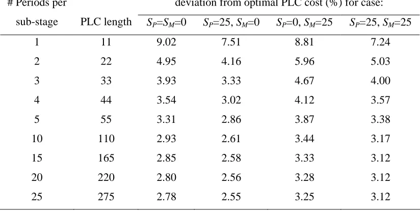
policy characterizations for the case where Sp=$25 & Sm=$25…………. 74 Table 5.12 The performance of the long-run policy characterizations over PLCs with

several lengths……… 76 Table 5.13 The percentage deviations from optimal PLC costs for no policy revision,

Table A.1 The effect of changing several cost parameters when lp=1 & lm=2……. 88 Table A.2 Results in the existence of non-zero manufacturing and remanufacturing

set up costs, SP and SM, when lp=1 & lm=2……… 89 Table A.3 The effect of changing several cost parameters when lp=2 & lm=1……... 90 Table A.4 Results in the existence of non-zero manufacturing and remanufacturing

set up costs, SP and SM, when lp=2 & lm=1………. 91 Table A.5 Policy characterizations under demand distributions with different CVs

for the case where lp =lm =1 and SP =SM =0……….. 92

Table A.6 Policy characterizations under demand distributions with different CVs for the case where lp =lm =1 and SP =10& SM =16……… 92

Table A.7 Policy characterizations under demand distributions with different CVs for the case where l_p =1 & l_m =2 and S_P =S_M =0……….. 93 Table A.8 Policy characterizations under demand distributions with different CVs

for the case where l_p =1 & l_m =2 and S_P =10&S_M =16……… 93 Table A.9 Policy characterizations under demand distributions with different CVs

for the case where lp =2 & lm =1 and SP =SM =0………. 94

Table A.10 Policy characterizations under demand distributions with different CVs for the case where lp =2 & lm =1 and SP =10&SM =16……… 94

Table B.1 The descriptions of the policy structures………... 95 Table B.2 The relevant inventory position definitions for manufacturing and

remanufacturing decisions under different lead time cases………... 95 Table B.3 The policy characterizations for the scenarios where Sp=Sm=0 and

lp=lm=1………96 Table B.4 The policy characterizations for the scenarios where Sp>0 & Sm=0 and

lp=lm=1………97 Table B.5 The policy characterizations for the scenarios where Sp=0 & Sm>0 and

Table B.6 The policy characterizations for the scenarios where Sp>0 & Sm>0 and

lp=lm=1………..100 Table B.7 The policy characterizations for the scenarios where Sp=Sm=0 and

lp=1 & lm=2……… 103 Table B.8 The policy characterizations for the scenarios where Sp>0 & Sm=0 and

lp=1 & lm=2………. 104 Table B.9 The policy characterizations for the scenarios where Sp=0 & Sm>0 and

lp=1 & lm=2……….. 105 Table B.10 The policy characterizations for the scenarios where Sp>0 & Sm>0 and

lp=1 & lm=2………. 107 Table B.11 The policy characterizations for the scenarios where Sp=Sm=0 and

lp=2 & lm=1……….. 110 Table B.12 The policy characterizations for the scenarios where Sp>0 & Sm=0 and

lp=2 & lm=1……….. 110 Table B.13 The policy characterizations for the scenarios where Sp=0 & Sm>0 and

lp=2 & lm=1………. 112 Table B.14 The policy characterizations for the scenarios where Sp>0 & Sm>0 and

lp=2 & lm=1……….. 113 Table B.15 The training data for group 1 for the case where lp=lm=1……… 117 Table B.16 The testing data for group 1 for the case where lp=lm=1………. 119 Table B.17 The predicted policies for the testing scenarios for group 1 for the case

where lp=lm=1………... 120 Table B.18 The training data for group 2 for the case where lp=lm=1……… 121 Table B.19 The testing data for group 2 for the case where lp=lm=1………. 123 Table B.20 The predicted policies for the testing scenarios for group 2 for the case

where lp=lm=1 .……… 125 Table B.21 The training data for group 1 for the case where lp=1, lm=2 ………….. 127 Table B.22 The testing data for group 1 for the case where lp=1, lm=2 ………. 129 Table B.23 The predicted policies for the testing scenarios for group 1 for the case

Table B.24 The training data for group 2 for the case where lp=1, lm=2 ………….. 131 Table B.25 The testing data for group 2 for the case where lp=1, lm=2 ………. 133 Table B.26 The predicted policies for the testing scenarios for group 2 for the case

where lp=1, lm=2 ……….. 135 Table B.27 The training data for group 1 for the case where lp=2, lm=1 …………... 137 Table B.28 The testing data for group 1 for the case where lp=2, lm=1 ………. 139 Table B.29 The predicted policies for the testing scenarios for group 1 for the case

where lp=2, lm=1 ………. 140 Table B.30 The training data for group 2 for the case where lp=2, lm=1 …………... 141 Table B.31 The testing data for group 2 for the case where lp=2, lm=1 ………. 143 Table B.32 The predicted policies for the testing scenarios for group 2 for the case

where lp=2, lm=1………... 145 Table C.1 The descriptions of the inventory policies………... 147 Table C.2 The cost sensitivity of the inventory policies for the case where

SP=SM=0………... 148 Table C.3 The cost sensitivity of the inventory policies for the case where SP=25,

SM=0………. 148 Table C.4 The cost sensitivity of the inventory policies for the case where SP=0,

SM=25………... 149 Table C.5 The cost sensitivity of the inventory policies for the case where SP=25,

LIST OF FIGURES

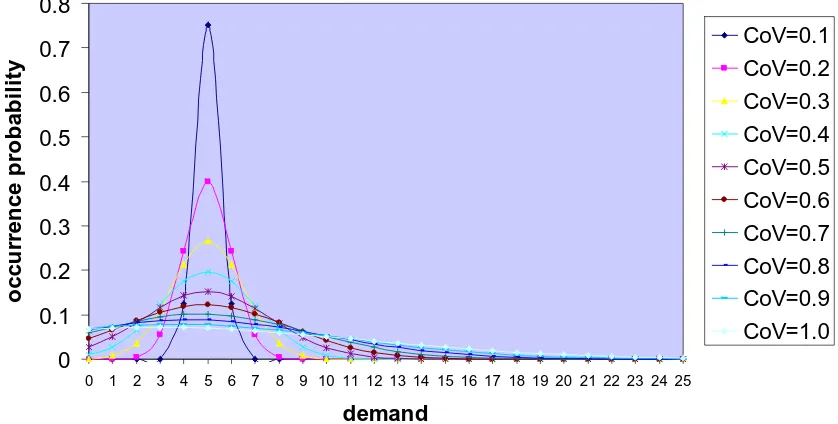
Figure 3.1 The recoverable manufacturing system……… 18 Figure 3.2 Demand distributions with μ =5 and coefficient of variations 0.1-1.0…39 Figure 5.1 Demand and return rates over a typical life cycle of a recoverable

1. Introduction

In recent years, manufacturers have paid growing attention to reuse activities that provide material waste reduction via the recovery of some content of used products. Motivation behind these product recovery activities is two-fold: growing environmental concerns and potential economical benefits. In several countries environmental

regulations are in place, which make manufacturers responsible for the whole life cycle of the product they produce. A common example of these regulations is take-back obligations after usage (Fleischmann et al., 1997). But even in the absence of such regulations, the expectations of environmentally conscious consumers put pressure on companies to consider environmental issues in their manufacturing process. Nowadays, a green image, which can be obtained by implementing recoverable manufacturing

systems, has become a powerful marketing tool and provides a significant competitive advantage to companies who seek to have a place in the global market. Reuse of products or materials can be economically attractive as well in addition to contributing to

sustainable development. Disposal costs have increased significantly in recent years due to depletion of incineration and land filling capacities. Companies are considering product recovery to avoid disposal cost. Further, with product recovery, not only savings in disposal cost are obtained but also the value incorporated in the used product is

regained, which provides energy, material and labor savings.

Recoverable manufacturing systems can be defined as closed loop systems with discarded items used in place of externally supplied virgin materials to the greatest extent possible in the fabrication of new products (Guide et al., 2000). These systems are

capable of dealing with product returns via several product recovery options, which can be categorized as direct reuse, repair, refurbishing, remanufacturing, cannibalization and recycling with respect to increasing degree of required disassembly level (Thierry et al., 1995). There are several review papers that emphasize the challenges of considering product recovery. Thierry et al. (1995) describe strategic issues that manufacturers face in implementing product recovery management policies. Fleischmann et al. (1997) provide a systematic review of reverse logistics issues and mathematical models for dealing with returns in distribution planning, production planning and inventory control areas. Guide et al. (2000) discuss the complicating characteristics of recoverable manufacturing systems including uncertainties in timing, quantity and quality of returns, the need for balancing demands with returns, disassembly need for returned products, the requirement of a reverse logistics network, material matching restrictions and stochastic routings for materials to be used in recovery operations.

Two main additional sources of complexity appear in inventory control of

recoverable manufacturing systems compared with traditional inventory systems without product returns. First, due to uncertainty of the product returns, an additional stochastic impact needs to be considered. Second, the product recovery option (e.g.

remanufacturing) must be coordinated with regular procurement (e.g. manufacturing), which complicates the inventory control situation.

In recent years, the challenges that are faced when dealing with returns in the context of production planning and inventory management have gained considerable attention of researchers. Consequently, studies regarding recoverable manufacturing systems have found a place in the literature, which are mentioned thoroughly in the next section.

remanufacturing are taken into consideration. Stochastic recoverable systems with similar characteristics have been widely investigated in the last decade; however, no work exists in the literature which conducts an analysis to find the optimal inventory policy structure in the existence of fixed cost for regular production and/or remanufacturing. Further, to our knowledge, none of the work that uses a pre-determined policy structure for

inventory optimization indicates how well the policy structure they consider characterizes the optimal inventory control policy.

This dissertation aims to find the structure of optimal inventory control policies for the recoverable manufacturing system under several cost configurations including non-zero set up costs for manufacturing and remanufacturing operations. The optimal inventory policies are found by solving the Markov Decision Process (MDP) model of the recoverable system, and an empirical study is conducted to determine policy characterizations under several cost configurations and lead time relations. The performance of the policy characterizations provided is evaluated numerically

considering the percentage deviation of their costs from the optimal cost. Based on the policy characterizations, it is investigated how the policy structure as well as policy parameter values change as cost parameters of the system change. Consequently, an MDP-based search procedure is introduced to determine inventory policy

characterizations given that appropriate policy structures under certain cost

configurations are known. Further, a neural network analysis is performed to determine the functional relationships between cost parameters of the system and the inventory policy parameter values. Finally, the optimal inventory policies are investigated through the entire product life cycle of a remanufacturable product. Benefiting from the long-run optimal policies found through MDP analysis, the optimal or near-optimal policy

2. Literature survey on inventory control in recoverable manufacturing systems

Traditional inventory models do not consider that manufactured items that are sold to the market may be returned to the manufacturer by the end users after a certain time and may need to be recovered by the manufacturer. Nowadays, many manufacturers take back their products from customers after their consumption, either due to responsibilities resulting from legislation or due to economic profits of product recovery (Inderfurth and Van der Laan, 2001).

Two main additional sources of complexity appear in inventory control of

recoverable manufacturing systems compared with traditional inventory systems without product returns. First, due to uncertainty of the product returns, an additional stochastic impact needs to be considered. Second, product recovery options (e.g. remanufacturing) must be coordinated with regular procurement options (e.g. manufacturing), which complicates the inventory control situation.

versus infinite horizon models, periodic review versus continuous review models, models with/without disposal option, etc.

A major classification observed in the literature is deterministic versus stochastic recoverable systems. Furthermore, stochastic product recovery models are classified into periodic versus continuous review models. In periodic review models, decisions

regarding inventory replenishment are made on a periodic basis while in continuous review models inventory levels are monitored continuously and decisions can be made at any time. The following two sections review several works on deterministic and

stochastic inventory systems with product recovery option, respectively.

2.1. Deterministic recoverable inventory models

In deterministic recoverable inventory models, all the components of the system (e.g., cost information, lead times, customer demand and product returns over the entire

planning horizon) are assumed to be known with certainty (Fleischmann, 2001). The deterministic recoverable models can primarily be subdivided into static and dynamic models. In the former, demands and returns are stationary. In other words, demand and return rates are constant over the planning horizon. While in the latter, demand and return rates are dynamic, i.e. they vary through time.

every external procurement order. The expressions for the optimal policy parameters are derived in an analogous way to EOQ model. Mabini et al. (1992) provide EOQ-type formulations for controlling inventory in a single item repairable system where stock outs are allowed up to a certain level. Their aim is to find the purchase and repair quantities that would minimize total cost while satisfying a certain service level. Furthermore, they extend their model to a multi-item situation where multiple items share a common limited repair capacity. Richter (1996) presents a deterministic two-stage EOQ model that

describes the production of new items and the repair of used items in a first shop and the employment of the new or repaired products in a second shop at a constant demand rate. At the end of a collection period, the used products in the second shop are either disposed of or brought back to the first shop for repair according to a certain repair rate. In addition to the fixed set up costs and the holding costs, the system cost includes the variable production, repair and disposal costs as well. More than one set ups for production and repair within the collection interval are allowed. One shall note that all the above mentioned works are common in the following sense: First, they all consider a

predetermined inventory holding policy without investigating its optimality. Second, a remanufactured or repaired item is assumed to be “as-good-as” a newly produced item in terms of quality. Third, the quality of the returned items is assumed to be perfect for reuse. More recently, Dobos and Richter (2006) investigate a production/recycling model with quality considerations. They show that it is better to outsource the quality control and repurchase only reusable products in order to minimize the total EOQ related (i.e. the fixed set up/order costs and the holding costs) and non-EOQ related (i.e. the linear waste disposal, recycling, production and repurchasing costs) costs.

Beside the static recoverable models, the dynamic recoverable models as well have received the attention of researchers. The variants of Wagner/Whitin algorithm (Wagner and Whitin, 1958) have been developed in the context of Reverse Logistics to solve dynamic recoverable models. For instance, Richter and Sombrutzki (2000) study the pure reverse Wagner/Whitin model and some of its extensions, where only the

remanufactured items. Furthermore, they analyze the model of alternate application of remanufacturing and manufacturing processes where both newly produced items and remanufactured items have the same value and can be used to satisfy customer demand. In a later work, Richter and Weber (2001) extend the reverse Wagner/Whitin model by incorporating the variable manufacturing and remanufacturing costs into the model. This model can be viewed as a combination of the classical Wagner/Whitin model and a pure reverse Wagner/Whitin model. They also investigate how the existence of a disposal option for used products would affect the solution.

2.2. Stochastic recoverable inventory models

Regarding stochastic inventory control problems in the existence of remanufacturing options, two streams of contributions can be found in the literature: one includes

periodic-review models, the other includes continuous-review models.

Two main approaches are observed in the literature regarding inventory management of stochastic recovery models. One approach, which has been rarely used, is to

investigate the structure of the optimal control policy using dynamic programming approaches (e.g., Simpson, 1978; Inderfurth, 1997). A second approach is to find optimal or near-optimal values for the parameters of a predetermined reasonable, but not

necessarily optimal, control policy structures, benefiting from the results of queuing theory, Markov decision processes, enumeration techniques, simulation or heuristics (e.g. Kiesmuller, 2003; Kiesmuller and Scherer, 2003; Kiesmuller and Minner, 2003;

2.2.1. Periodic-review models

Periodic review models describe practical situations in a more suitable way. However, only a few papers can be found in the literature which considered periodic review models in the context of product recovery. Furthermore, the majority of these investigate the optimal parameter values for a pre-determined policy rather than finding the optimal policy structure itself for the system under consideration. Kiesmuller (2003) considers a pre-determined periodic review PULL policy, named as (S, M) policy, for a stochastic hybrid manufacturing/remanufacturing system with two stocking points without a disposal option and with different lead time cases for manufacturing and remanufacturing operations. The key point in their approach is defining different inventory positions on which production and remanufacturing decisions will be based. They provide a comparative analysis to justify the use of separate inventory position definitions for production and remanufacturing decisions rather than using a single inventory position definition for both decisions. They calculate optimal parameter values of the pre-determined policy and the optimal cost using grid search and simulation. Kiesmuller and Minner (2003) provide simple Newsvendor type heuristic formulae to calculate the parameter values of the (S, M) policy. Their numerical study shows that the proposed formulae lead to near optimal parameter values in most cases. Mahadevan et al.

(2003) employ a periodic review push policy, named as (R, S) policy, to analyze a similar recoverable inventory system. They develop several heuristics based on traditional

models to find the values of this pre-determined policy’s parameters.

for which he uses the method of stochastic dynamic programming to derive optimal decision rules for procurement, remanufacturing and disposal. He explores the impact of procurement and remanufacturing lead times to the complexity of the optimal decision rules and shows that up to a certain extent, simple rules with only a few parameters can be proved to be optimal for the stochastic recovery problem. For the case without stock keeping of recoverable items, he formulates optimal policy structures for different lead time cases. In addition, for the stock keeping of recoverable items case, he provides the optimal policy structure only for the case of equal lead times and no set up cost for production and remanufacturing. Inderfurth indicates that if there existed fixed costs of remanufacturing or normal production, the policies may no longer be optimal.

Kiesmuller and Scherer (2003) consider the optimal policy structures provided by Inderfurth (1997) for one product recovery system with/without stock keeping of returns under equal lead times for manufacturing and remanufacturing, and provide a method for exact computation of the policy parameters and a couple of heuristic methods.

2.2.2. Continuous-review models

The first continuous review model for the manufacturing systems with product returns was proposed by Heyman (1977). Heyman considers a single item continuous-review inventory model with stochastic uncorrelated demand and returns. A returned item is either disposed of or repaired upon arrival. He disregards the fixed cost of ordering (implying no lot size reordering) and assumes instantaneous procurement and repair (implying no backorders or lost sales). Under these assumptions, he optimizes a single parameter policy that consists of only a disposal level, which is defined as the serviceable inventory at which returned products are disposed of.

which an outside procurement order of Q units is placed. Closed form expressions for calculating reorder level, r, and order quantity, Q, are provided. Further, the results of the single echelon case are extended to a specific two echelon case where a warehouse (upper echelon) supports several retailers (lower echelon).

Vander Laan et al. (1995) propose two control policies, namely (sm, Qm, Qr) PUSH and (sm, Qm, sr, Sr) PULL strategies for inventory control of hybrid manufacturing and remanufacturing systems without a disposal option for returned items. Although these strategies are non-optimal, they have the advantage that they are easy to implement and they are actually used in practice. The two strategies are the same in terms of

manufacturing decision. According to both strategies, when serviceable inventory position is below sm, a manufacturing order of size Qmis placed. The main difference between PUSH and PULL strategies is that with PUSH control, returned products are remanufactured as early as possible while with the other, they are remanufactured as late as possible. Under PUSH control, returned products are pushed into the remanufacturing process every time recoverable inventory reaches a certain level (i.e. Qr) while under PULL control, remanufacturing operations do not start unless the serviceable inventory position is sufficiently low (i.e. below sr) and there are enough returned items in

recoverable inventory to increase the serviceable inventory position up to a certain level,

Sr.

Van der Laan et al. (1996) consider a single product single echelon remanufacturing system with product disposals where outside procurement is considered as a second supply mode in addition to remanufacturing to meet demand. Lead time for outside procurement is deterministic while remanufacturing lead time is stochastic. There is a fixed outside procurement cost per order and variable outside procurement cost per ordered unit of product. No fixed cost is considered for remanufacturing. There are c

parallel machines for remanufacturing, and once one become available, a returned item in queue is pushed into remanufacturing. When there is no room in queue for

respect to disposal control rule. Note that the last two policies are a special case of (sp,Qp,sd,N) policy. According to (sp,Qp,sd,N) policy, the strategy with respect to outside procurement is: whenever inventory position, which consists of net serviceable inventory, returned items in the remanufacturing facility and outside procurement orders, drops to sp an outside procurement order of Qp units of products is given. The strategy with respect to remanufacturing or disposal is whenever the number of returned items in

remanufacturing facility is N or the serviceable inventory equals sd, returned units are disposed of upon arrival. In order to calculate expected cost for pre-determined policies, Van der Laan et al. (1996) employ an analytical procedure that requires formulating and solving a continuous-time Markov chain model with two state variables, inventory position and the returned items in the remanufacturing facility. They use an enumerative search procedure to find the optimal parameter values for the policies under

consideration. Via a numerical study, they show how the performance of each policy varies when the return rate or the remanufacturing rate changes. In a later study, Van der Laan and Salomon (1997) consider a manufacturing/remanufacturing system with planned disposal operations where customer demands and returns are correlated. Inter-arrival times for demand and return are Coxian-2 distributed. Both remanufacturing and production have deterministic non-zero lead times. They extend PUSH and PULL strategies that Vander Laan et al. (1995) developed for a similar system without planned disposal option to PUSH-disposal and PULL-disposal strategies that include one

additional parameter, i.e. sd, which defines disposal strategy. Through numerical examples, they provide a comparison between systems with and without disposals, a comparison between PUSH-disposal and PULL-disposal strategies, and a study on the robustness of control parameters over the different stages of product life cycle. Later, Van der Laan et al. (1999a) consider a single product hybrid

manufacturing/remanufacturing system without disposal option where manufacturing and remanufacturing lead times are modeled as deterministic as well as a discretely

system. They model the system under consideration as a continuous-time Markov chain model and use an enumerative search procedure to find the optimal control parameters (or, optimal cost) for PUSH and PULL policy. Similarly, Van der Laan et al. (1999b) present an exact methodology that requires an extensive enumerative search to optimize a PUSH control strategy and a PULL control strategy. Through a numerical study, they compare the cost of a traditional inventory system without remanufacturing operations that is controlled by a simple (s, S) policy to the costs of hybrid

manufacturing/remanufacturing systems controlled by a PULL or a PUSH policy. Furthermore, they compare the cost of a PUSH controlled system to a PULL controlled system under several scenarios.

Inderfurth and Van der Laan (2001) investigate the information structure (inventory information necessary for optimal stock replenishment) of a predetermined control policy from a theoretical point of view. They consider a simple 4-parameter control policy and show that the performance of the policy can be improved considerably if the inventory information to consider when making a production decision is defined appropriately.

Fleischmann et al. (2002) consider a basic single-echelon inventory model where there is no distinction between new and returned items in terms of quality. Returned items upon arrival join directly serviceable item stock without requiring any recovery operations. In addition to returned items, new items that are obtained by outside procurement are also used to meet customer demand. They show the optimality of the conventional (s, Q) policy for ordering new items under the assumption of stochastic demand and returns, and they provide a procedure to calculate optimal control

stochastic inventory model where demand can take both positive and negative values, a negative demand representing the arrival of a returned item. Benefiting from the general theory of Markov decision processes, they show the average cost optimality of an (s, S) policy. Through a numerical study, the effect of return flow on the system costs (fixed cost, holding cost and backordering cost) is investigated.

More recently, Van der Laan and Teunter (2006) consider PUSH and PULL

remanufacturing policies to control a hybrid inventory system with unit product returns and demands where the remanufacturing option is cheaper than the manufacturing option. The system costs include set up costs, holding costs and backordering costs. They

develop simple closed form expressions for calculating near-optimal parameter values for these policies, and in an extensive numerical study, they evaluate the performance of the proposed heuristics by comparing their costs to the costs associated with optimal

3. Inventory Optimization for a Periodically-Reviewed Recoverable Manufacturing System

Recoverable manufacturing systems can be defined as closed loop systems with discarded items used in place of externally supplied virgin materials to the extent possible in the fabrication of new products (Guide et al., 2000). These systems are capable of dealing with product returns via several product recovery options, e.g. direct reuse,

repair, refurbishing, remanufacturing, cannibalization and recycling (Thierry et al., 1995). We consider here a periodically-reviewed recoverable system where remanufacturing is used as the recovery option. In addition to newly produced items, remanufactured items as well can be used to meet customer demands. Remanufactured items are considered to have the same quality as the new products and are sold for the same price, but they are less costly.

Two main approaches are observed in the literature regarding inventory management of stochastic recovery models. One approach, which has been rarely used, is to

analytically investigate the structure of optimal control policies using dynamic

programming approaches (e.g., Simpson, 1978; Inderfurth, 1997). A second approach is to find optimal or near-optimal values for the parameters of a predetermined reasonable, but not necessarily optimal, control policy structure, benefiting from the results of queuing theory, Markov decision processes, enumeration techniques, simulation or heuristics (e.g. Van der Laan et al. 1996; Van der Laan and Salomon, 1997; Van der Laan et al. 1999; Kiesmuller, 2003; Kiesmuller and Minner, 2003; Kiesmuller and Scherer, 2003; Mahadevan et al., 2003; Van der Laan and Teunter, 2006). The latter approach has been widely used for both periodically and continuously reviewed recoverable inventory systems due to its simplicity and its applicability to more comprehensive, larger-scale models with relaxed assumptions compared to models to which the former approach has been applied. However, it has the drawback of considering a pre-determined policy that is not guaranteed to be optimal. In these works, it is not indicated how far the

predetermined policy is from the optimal policy.

in the context of product recovery. Further, the majority of these investigate the optimal parameter values for a pre-determined policy rather than finding the optimal policy structure itself for the system under consideration (Kiesmuller, 2003; Kiesmuller and Minner, 2003; Mahadevan et al., 2003) To our knowledge, only a couple of papers in the literature emphasize the generation of optimal control policy structures for a one product recoverable system. Simpson (1978) generates the optimal policy structure for a finite-horizon repairable inventory problem under no set up costs and zero lead time

assumption for repair and purchasing activities. He uses a backward dynamic programming technique. Inderfurth (1997) addresses the problem of inventory

optimization for a recoverable system with and without stock keeping of returned items for which he uses the method of stochastic dynamic programming to derive optimal decision rules for procurement, remanufacturing and disposal. For the case where recoverable items are stocked, he provides the optimal policy structure only for the case of equal lead times and no set up costs for manufacturing and remanufacturing. He indicates that if fixed costs exist, the policies provided may no longer be optimal.

To our knowledge, no work exists in the literature which conducts an analysis to find optimal policy structure in the existence of fixed costs for manufacturing and/or

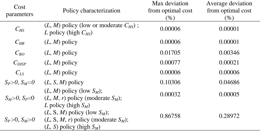
This chapter considers inventory optimization problem of a periodically reviewed single product stochastic manufacturing/remanufacturing system with two stocking points: recoverable inventory and serviceable inventory. Lead times and set up costs for manufacturing and remanufacturing are considered. The system is modeled using Markov Decision Process, and an empirical study is conducted to determine optimal or near optimal policy characterizations under several cost configurations and different lead time cases for manufacturing and remanufacturing. Through these policy characterizations, how the optimal policy structure and/or policy parameter values change as several cost parameters including set up costs change is investigated. The performance of the policy characterizations provided under several cost configurations is evaluated numerically considering the percentage deviation of their cost from the optimal cost. Results indicate that the existence of set up cost for either manufacturing or remanufacturing has a significant effect on policy structure, and the policy characterizations we provide

represent the optimal policies well with a maximum deviation of 1% from optimal cost in almost all cases.

This chapter is organized as follows: In section 3.1, the recoverable manufacturing system under consideration is presented and the inventory optimization problem is formulated as a discrete Markov Decision Process under different cases for

manufacturing and remanufacturing lead times. In section 3.2, the experiments to be performed are described. In section 3.3, the effects of a change in cost parameters of the system on the optimal inventory policies are investigated through policy

characterizations. Sections 3.3.1, 3.3.2 and 3.3.3 include the optimal or near-optimal policy characterizations determined under several cost configurations for the three lead time cases considered, i.e. the case where manufacturing and remanufacturing lead times equal one period; the case where remanufacturing lead time is two periods and

manufacturing lead time is one period; and the case where manufacturing lead time is two periods and remanufacturing lead time is one period, respectively. Further, in section 3.4, sensitivity analysis is provided regarding the effect of changing the coefficient of

3.1. Problem description and MDP formulations

This chapter considers a one product stochastic manufacturing/remanufacturing system with two stocking points: serviceable inventory and recoverable inventory, as illustrated in figure 3.1. Serviceable inventory includes finished products that are ready for sale while recoverable inventory includes no longer needed used products returned to manufacturer, which are considered for remanufacturing. Serviceable inventory can be replenished in two ways: one is the production of new items using externally supplied new materials or parts, which will be referred from now on as regular production or

manufacturing. The other is the recovery of returned items via remanufacturing. A remanufactured product is considered as a ‘like new’ item that has the same quality and price as a new one.

Recoverable Inventory

Serviceable Inventory

Regular Production/ Manufacturing

p

J

I

m

Remanufacturing

D

Demand

R

Return

Disposal

Figure 3.1. The recoverable manufacturing system

Demand and returns per period are stochastic, and they are represented using discrete-type bounded probability distributions. Customer demands during a given period are satisfied from the serviceable items on hand at the beginning of that period. Backordering of non-satisfied demands is allowed up to a certain level, beyond which an incoming demand is lost.

Recoverable inventory has a finite capacity. When the recoverable inventory is full, incoming returns are disposed. Other than this situation, the disposal option for returned items is not considered as a part of manufacturer’s decision. A justification of this assumption is that disposal would be necessary only when product return rate is very large relative to demand rate and special cost parameters exist (Teunter and Vlachos, 2002). On the other hand, our approach can be easily extended to include a disposal option into the system.

The inventory optimization problem regarding this recoverable system is to find the optimal policy that defines how many items to manufacture and remanufacture given serviceable and recoverable inventory levels and manufacturing or remanufacturing work-in-process. A policy is considered to be optimal if it provides the smallest expected cost per period.

The system is formulated as a discrete-time Markov Decision Process (MDP) to find the optimal policy. A Markov Decision Process model is a stochastic sequential-decision model that is defined by a set of system states, a set of decisions to make, immediate reward function to optimize and transition probability matrix that defines the probability of going from one state to another in one transition under a selected decision (Puterman, 1994). The MDP model of the recoverable manufacturing system is formulated as follows:

State space

max min I I I ≤ t ≤

max 0≤ Jt ≤J

where and represent net serviceable inventory (i.e., on-hand serviceable inventory minus backorders) and recoverable inventory at the beginning of period t, respectively, and if , that means, backordering of the demand up to –I

t

I Jt

0

min <

I min units is

allowed.

For the cases where manufacturing or remanufacturing has a two-period lead time, a third state variable is needed, which represents the work in process (WIP) associated with the order regarding the operation with two-period lead time that is initiated at the

beginning of previous period. Clearly, for state feasibility, the following constraint must be satisfied every period:

max I Z I_t + _t ≤

where is the order regarding the operation with two-period lead time that is given at the beginning of period t-1 and that will be ready at the end of period t. will be referred as the serviceable inventory position at the beginning of period t before any manufacturing or remanufacturing decision has been made, hereafter.

t

Z

t

t Z

I +

Decision space

Decisions to be made are how many items to manufacture and remanufacture at the beginning of each period. Clearly, the decisions are based on the system state at that time. Manufacturing and remanufacturing capacities of the manufacturer are considered to enable the modeling of capacitated problems. Note that these capacities can be set sufficiently large to fit the problems with no capacity restrictions as well.

Say the beginning-of-period serviceable and recoverable inventory levels, and , and WIP regarding the operation with two-period lead time, , form the state . For state , the feasible pairs of regular production and remanufacturing decisions are calculated as follows.

t

I Jt

t

Z S_t

t

S

inventory and replenishes serviceable inventory, hence the manufacturer should choose a remanufacturing amount considering the number of returned items on hand, the

remanufacturing capacity, as well as the serviceable inventory storage capacity. As a result, a feasible remanufacturing decision, say m, can take the following values for stateSt:

_{m m}St (1) max , , 1 , 0 _K =

}

}

where ; represents the largest feasible remanufacturing amount that can be ordered when the system state is and

represents the remanufacturing capacity of the manufacturer.

{

S Z I I M J

m t = − −

max max

max min , ,

t S mmax t S max M

Similarly, the production decision, say p, must be made considering the serviceable inventory storage and regular production capacities. Given that the remanufacturing decision is m, a feasible regular production decision can take the following values:

_{p p}St (2) max , , 1 , 0 _K =

where ; represents the largest feasible regular production amount that can be ordered when the system state is and

represents the regular production capacity of the manufacturer.

{

max min I I Z m, P

pSt = − _t − _t − _pSt

max

t

S

max P

Clearly, if the lead times equal one period for both operations, the term equals 0 in the above formulations since no work in process is available for this case. Consideration of (1) and (2) together yields a feasible pair of regular production and remanufacturing decisions, (p, m), for state S

t

Z

t.

State transition and transition probabilities

State transition from the current period to next depends on manufacturing and remanufacturing decisions made, as well as, customer demands and returns that occur in current period. Hence, given that the current state is St=(It, Jt, Zt), the manufacturing and remanufacturing decisions taken are p and m, and demand and return during period t,

and , take the values d and r, respectively, the next state will be S

t

D Rt t+1=(It+1, Jt+1,

{

}

{

}

{

}

{

}

1 min J m r,J J_t+ = _t − +

⎪ ⎭ ⎪ ⎬ ⎫ ⎪ ⎩ ⎪ ⎨ ⎧ = = = = = = = + 1 if 0 2 , 1 if 1 2, if 1 m p m p m p t l l l l m l l p Z

The transition probability from Stto St+1 under decision (p, m), represented by , equals the sum of the probabilities of occurrence for the pairs of demand and return, (d,r), that lead to transition from S

)) , ( , ,

(S S ₁ p m P _{t t+}

tto St+1under the decision (p, m), as indicated below.

∑

1,( , )) ( )* ( )

, ( m p t S t S A r d t t t

t S p m P D d P R r

S P

where Dt and Rt represent demand during period t and the number of items returned to manufacturer during period t, respectively, and is the set that includes the pairs of demand and return that make the system go from S

) , ( 1 m p S S_{t t}

A _{→ +}

tto St+1under the decision (p, m). Reward function

The reward function to optimize for this problem is defined as the expected cost per period, which consists of fixed and variable manufacturing and remanufacturing cost, holding cost for serviceable and recoverable inventory, holding cost for work-in-process, backordering cost, lost sales cost and disposal cost. The following notation is used for the cost function.

SP : setup cost for manufacturing,

SM : setup cost for remanufacturing

P

C : unit manufacturing cost

M

C : unit remanufacturing cost

HS

C : holding cost per serviceable unit or unit WIP per period

HR

C : holding cost per recoverable unit per period

BO

DISP

C : unit disposal cost for recoverable items

LS

C : unit lost sales cost

t

DISP: disposal amount during period t

t

LS : lost sales during period t

:

t

B backordered demand during period t

Given that the system is in state St , manufacturing and remanufacturing decisions

taken are p and m, respectively, and d units of demand and r units of returns occur during period t, the cost during period t is calculated as:

[ ]

+1 1 1

) ( ) ( )) , ( ), , ( , ( δ γ

where the terms represent manufacturing cost, remanufacturing cost, holding cost for serviceable inventory, holding cost for work in process (if any), holding cost for

recoverable inventory, backordering cost, disposal cost, and lost sales cost (or, lost sales revenue), respectively, and

⎩ ⎨ ⎧ = > + = 0 0 0 ) ( p for p for p C S

p P P

δ , ⎩ ⎨ ⎧ = > + = 0 0 0 ) ( m for m for m C S

m M M

γ

[ ]

{

+

+ = t

t I

I

}

{

}

{

}

⎩ ⎨

⎧− − − <

= otherwise I d I if I d I

Bt t t

0

0 ,

max ,

max _{min min}

⎩ ⎨

⎧ − + − − + >

= otherwise J r m J if J r m J

DISP_t t t

0 max max

[

]

[

]

⎧ − − − <

= otherwise I d I if d I I

LSt t t

0

min min

Then, the expected cost to occur in period t is calculated considering all possible pairs of demand and return, as:

[

]

_∑∑

r d

t t

t

t p m P D d R r C S p m d r

S C

The MDP model formulated is solved using a variant of Howard’s policy iteration method that integrates the fixed policy successive approximation presented by Morton (1971). Howard’s policy iteration method (Howard, 1960) for infinite horizon MDP problems is a two-phase method consisting of the alternate use of value determination and policy improvement stages until no more improvement is obtained. A disadvantage of Howard’s policy iteration method is that it requires solving N simultaneous linear equations in every iteration to determine the relative values of given policy, N

representing the number of states. This may require huge computational effort and/or lead to excessive computer round off errors, which makes large MDPs computationally intractable. Morton’s approach differs by Howard’s in that relative values are computed by the fixed policy successive approximation, which eliminates the need for solving linear equations (Morton, 1971). It is worth while noting that the successive approximation concept was introduced by White (1963) as an alternative to Howard’s approach, and shown empirically to be computationally more efficient.

3.2. Experiments setting and the analysis

The recoverable manufacturing system described in the previous section is

investigated under several cost configurations that are generated from a so-called basic scenario by changing the value of a single cost parameter at a time. Our objective behind these experiments is to find the effect of changing an individual cost parameter on the optimal inventory control policy.

The basic scenario considered for the recovery model under consideration is

described as follows: Demand and returns per period are represented using the following discrete-type bounded trapezoidal and triangular-shape probability functions,

The bounding constraints on serviceable and recoverable inventories are provided below:

30 10≤ ≤

− I_t for ∀t 0≤J_t ≤4 for ∀t

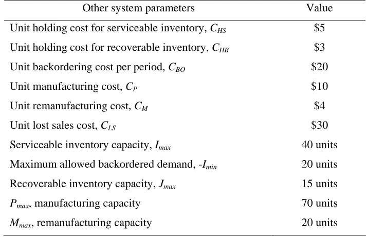
The capacities on regular production, Pmax, and remanufacturing, Mmax, are set to be 50 and 20 units per period, respectively. Note that these capacity values are relatively large, which allow us to find the optimal manufacturing/remanufacturing strategies under no capacity restrictions.

The values of the cost parameters in the basic scenario are determined considering the numerical data provided in Kiesmuller and Scherer (2003) except for lost sales cost which was not considered in their analysis. The cost parameters have the following values in the basic scenario:

0 = P

S , S_M =0, C_P= 10, C_M= 4, C_HS= 5, C_HR= 3, C_BO= 20, C_DISP= 0, C_LS= 30

The values of the cost parameters for the experimentation are arbitrarily selected, which are reported in Table 3.1. As can be seen from Table 3.1, extremely small or large values for the cost parameters are included in the experiments in order to see the optimal inventory policies in extreme cases as well. Note that the values in bold correspond to the cost parameters of the basic scenario.

Considering the values reported in Table 3.1, 30 new scenarios are created by

changing the value of a single cost parameter in the basic scenario. For each scenario, for every lead time case under consideration, the following methodology with 3 main steps is performed to find a good characterization of the optimal policy.

1. find the optimal policy by solving the MDP model

100 * 1 cost

optimal

zation characteri policy

of cost cost

optimal from

deviation

% _⎟⎟

⎠ ⎞ ⎜⎜

⎝ ⎛

− =

Table 3.1. The cost parameters and the corresponding values considered in the experiments

Cost parameters Values

Unit holding cost for serviceable inventory, CHS 1 3 5 10 20 30

Unit holding cost for recoverable inventory, CHR 1 3 5 10 20 30

Unit backordering cost per period, CBO 1 5 10 20 30

Unit disposal cost, CDISP -2 0 2 4.5

Unit lost sales cost, CLS 0 10 20 30

Set up cost for regular production, SP 0 10 20 30

Set up cost for remanufacturing, SM 0 2 4 8 12 16 24 40

Once policy characterizations are determined, the effects of changes in the values of cost parameters on the optimal policy structure and policy parameter values are analyzed individually.

3.3. Results regarding policy structures under different lead time cases

This section reports the results of the experiments described in the previous section under three different lead time cases. In the first lead time case, both manufacturing and remanufacturing operations have a one-period lead time. In the second lead time case, remanufacturing lead time is two periods and manufacturing lead time is one period. In the third lead time case, manufacturing has a two-period lead time and remanufacturing has a one-period lead time.

3.3.1. Results for unity lead time case for both manufacturing and remanufacturing

parameters’ values) provided regarding the optimal policy and the percentage deviations of their cost from optimal cost.

The optimal policy regarding the basic scenario is perfectly characterized using a two-parameter policy, named as the (L, M) policy, where L=13 and M=15, which has the optimal cost of $96.57.

Control rules regarding the (L, M) policy (where L<M) are described as:

• If I_t +J_t <L, then m= J_t(i.e., remanufacture all returned items on hand), and (i.e. manufacture up to L)

) (I m L

p= − _t +

• If L≤I_t +J_t <M, then m=J_t and p=0 (i.e., do not use regular production) • If I_t +J_t ≥M and I_t <M , m=M −I_t(i.e., remanufacture up to M) and p=0 • If I_t +J_t ≥M and I_t ≥M, m=0 and p=0

where and represent net serviceable inventory and recoverable inventory levels at the beginning of the period t, respectively, while p and m represent, respectively, how many items to manufacture and remanufacture.

t

I J_t

As can be noticed from the above rules, the parameters L and M represent

manufacture-up-to-level and remanufacture-up-to-level, respectively. A more compact description for the (L, M) policy would be:

Regarding remanufacturing: remanufacture up to M

{

}

⎩ ⎨

⎧ − <

= otherwise M I for I M J

m t t t

0 , min

Regarding manufacturing: manufacture up to L given m

⎩ ⎨

⎧ − + + <

= otherwise L m I for m I L

p t t

0

) (

significantly low expected disposal amount per period. Hence, the bounds put on the inventories are sufficiently large, which makes our recovery model behave like the model considered by Inderfurth (1997).

As can be observed from Tables 3.2 and 3.3, a change in the unit holding cost for serviceable items or recoverable items does not change the structure of the optimal policy, but it changes the optimal values of the policy parameters. The (L, M) policy structure is optimal for all values considered for unit serviceable holding cost except one, for which the deviation from optimal cost is only 0.00008%. Similarly, the (L, M) policy is optimal for all values considered for unit recoverable holding cost except one, for which the deviation from optimal cost is about 0.0011%.

From Table 3.2, we observe that as the unit serviceable holding cost increases, the values of L and M decreases. The optimal policy says to manufacture and remanufacture up to a lower level in order to decrease the expected end-of-period serviceable inventory level, because it gets more expensive to hold it.

Table 3.3 shows that an increase in unit holding cost for recoverable inventory results in an increase in the value of M. The optimal policy says to remanufacture up to a higher level in order to decrease the expected end-of period recoverable inventory. On the other hand, the value of manufacture-up-to-level, L, is not affected by a change in unit holding cost for recoverable inventory since manufacturing decision does not affect the

recoverable inventory level.

Table 3.2. The effect of changing holding cost for serviceable items, CHS, when lp=lm=1

CHS

Policy characterization

Table 3.3 The effect of changing holding cost for recoverable items, CHR, when lp=lm=1

CHR

Policy characterization

Deviation from optimal cost (%) 1 (L=13, M=14) 0.00108 3 (L=13, M=15) 0.00000 5 (L=13, M=17) 0.00000 10 (L=13, M=27) 0.00000 20 (L=13, M=27) 0.00000 30 (L=13, M=27) 0.00000

The (L, M) policy characterizes the optimal policy very well for the backordering cost values considered as can be seen from Table 3.4, the maximum deviation from optimal cost being only 0.02%. As the unit backordering cost decreases, the optimal values for parameters L and M decrease, because it becomes less costly to allow more backordering by manufacturing or remanufacturing up to a lower level, which will provide savings in holding cost. Note that there is a tradeoff between expected holding cost and expected backordering cost, i.e. the attempt of reducing one results in an increase in the other.

Table 3.4. The effect of changing backordering cost, CBO, when lp=lm=1

CBO

Policy characterization

Deviation from optimal cost (%) 30 (L=14, M=16) _0.00000 20 (L=13, M=15) _0.00000 10 (L=11, M=14) _0.00000 5 (L=8, M=12) _0.00000 1 (L=5, M=8) _0.01969

Table 3.5. The effect of changing disposal cost for recoverable items, CDISP, when lp=lm=1

CDISP

Policy characterization

Deviation from optimal cost (%) -2 (L=13, M=15) _0.00000

Table 3.6. The effect of changing lost sales cost, CLS, when lp=lm=1

CLS

Policy characterization

Deviation from optimal cost (%) 30 (L=13, M=15) _0.00000 20 (L=13, M=15) _0.00000 10 (L=13, M=15) _0.00000 0 (L=13, M=15) _0.00000

From Tables 3.5 and 3.6, we see that changing unit disposal cost or lost sales cost over a reasonable range does not have a significant effect on the optimal policy. Under the optimal policy for the basic scenario, i.e. the (L=13, M=15) policy, no lost sales occur and expected disposal amount per period is extremely low, and changing unit disposal cost or lost sales cost does not change this result. This indicates that the bounds put on the system inventories are sufficiently large so that they do not restrict the decisions.

From Tables 3.7 and 3.8, it can be clearly seen that the existence of set up cost for regular production or remanufacturing has a significant effect on the optimal policy structure. When there is non-zero set up cost for manufacturing, two parameters are needed to characterize the optimal manufacturing strategy, namely reorder level L and manufacture-up-to level S. According to this strategy, if serviceable inventory after the remanufacturing decision has been made is less than L (i.e.I_t +m<L), then an amount that will increase the serviceable inventory to S is manufactured, S being greater than L.

Table 3.7. The effect of changing set up cost for regular production, SP, when lp=lm=1

SP

Policy characterization

Deviation from optimal cost (%) 0 (L=13, M=15) _0.00000 10 (L=11, S=14, M=15) _0.00212 20 (L=10, S=15, M=16) _0.00018 30 (L=10, S=16, M=16) _0.00441

Table 3.7 shows that the (L, S, M) policy represents the optimal policy well in the case where there is set up cost for manufacturing but not for remanufacturing, the