Session Based Hidden Markov Model for
Network Anomaly Detection
Preetam U.Vernekar1, Dr.Rekha Bhandarkar2
Student, Dept. of E&C, NMAMIT, Nitte, Udupi District, Karnataka, India1
Professor, Dept. of E&C, NMAMIT, Nitte, Udupi District, Karnataka, India 2
ABSTRACT: Due to tremendous growth in Information technology, lead in the increase of threats from attackers for
several advantages. The most popular cyber threats occurring presently are Denial of Service and Distributed Denial of Service attacks. Intrusion Detection System is used to detect and prevent the malicious behaviour in network traffic where anomaly detection approach is used as the key element to discriminate normal and abnormal behavior of network traffic, hence referred as an intelligent security system. In this paper, Hidden Markov Model is used to detect potential anomalies in the network traffic which results in improved accuracy and maximizes detection rate.
KEYWORDS:Cyber Security, Network Intrusion Detection, DDoS, Hidden Markov Model
I. INTRODUCTION
Markov Model has been applied to anomaly detection mechanism inorder to classify the TCP network traffic asmalicious or normal.
II. RELATEDWORK
Sung-Bae Cho and Hyuk-Jang Park [7] present an optimal measure abstraction method based on a Hidden Markov Model to improve the models proposed by S.Forrest. They analyzed various attack patterns and enhanced system performance of HMM-based anomaly detection systems. The basic idea is to use privilege transition flows for modelling Hidden Markov Models so as to improve the intrusion detection rate while minimizing the false alarm rate. German Florez-Larrahondo [8] uses a novel incremental learning algorithm to allow Hidden Markov Models online learning from complex computer applications so as to generate the efficient anomaly detection models. All research on Hidden Markov Models is almost concentrated on anomaly detection. On the other hand, Hidden Markov Models are also used to represent the likelihood of transitions between security states [9]. Zhang Song-hong [10] uses Hidden Markov Models to model multi-step complex network attacks and to recognize the attacker's intention and to forecast next possible attack using the Forward and Viterbi algorithm. The perfect method and techniques for modelling complicate network attacks effectively have not been reported up to now.
III. HIDDENMARKOVMODEL
A Hidden Markov Model (HMM) is a statistical Markov Model with unknown parameters [5], and the challenge is to predict the hidden states based on the assumptions from the observable parameters.HMM are powerful statistical models for modelling sequential or time-series data.The HMM uses the property of Markov chains in which the probability of each present state depends on its previous state [5]. Transition from one state to another state emits an output which is an observable generated with respect to the probability distribution function. In HMM, the states are not visible to the observer only the outcomes are visible and therefore it is called as HMM.
Elements of HMM
N= Number of Hidden states represented as{S1,S2……SN}
K= Number of Observation symbols represented as {O1, O2…..Ok}
Initial probabilities π = (πi), where πi= π (Si) for i=0,1,.N-1
State Transition probability distribution A=aij where aij= P(Si at t+1|Sj at t) for i,j=0,..,N-1
Observation probability distribution with {Vk}set of output symbols B=bj(Vk) wherebj(Vk)=P(Vkat t|Sj at t)
We consider the system process as a first order Hidden Markov process, described by the model λ= (A, B, π). The fundamental issue is to resolve the problem of determining the best model λ= (A, B, π) that maximizes the conditional probability of the observation O given modelλ. Initial values of HMM parameters π, A, and Bare carried out to be uniformly distributed for each distinguishable TCP service. The transition probabilities can be estimated iteratively by means of the Baum-Welch algorithm. Baum-Welch algorithm uses the forward and backward algorithms to calculate the auxiliary variables α, β. Issues in HMM occurring are evaluation,decoding and training problem which are resolved using the algorithm mentioned below
Forward Algorithm: The forward variable αt(i) demonstrates probability of the partial unknown observation sequence
O, and state Si at time t , given the model λ . The main stages involved in Forward Procedure are
Initialization
( ) = ( )where = 0,1, . . −1, = 1,2. . . −1 (1) Induction
+ 1( ) = [ ∑ ( ) ] ( + 1) where , = 0,1, . . −1 and = 1,2. . . −1. (2) Termination
( | ) = ∑ ( ) where = 0,1, . . −1 (3)
Backward Algorithm:The Backward variable βt(i) defines the conditional probability of the partial observation
sequence from Ot+1to the end given state Siat time t and the model λ. The main stages involved in Backward Procedure
are
Initialization
Induction
( ) = [ ∑ + 1( ) ] ( + 1) where , = 0,1, . . −1 and = −1, −2. . . .1 (5)
Viterbi Algorithm: The Viterbi algorithm is a dynamic programming algorithm that computes the most likely state
transition path given an observed sequence of symbols. δt(i) is the probability of the most probable path ending in state Si at time t denoted as δt(i)=P(O/λ). Q gives the optimalstate probability. The main stages involved in Viterbi Procedure
are
Initialization
( ) = ( )where = 0,1, . . −1 (6)
Recursion
+ 1( ) = [ ( ) ] ( + 1)where , = 0,1, . . −1 and = 1,2. . . −1 (7)
Termination
= [ ( )] where = 1,2 … . . −1 (8)
Baum-Welch Algorithm: Baum-Welch Algorithm is used for estimating HMM parameters.
Re-estimating Initial state probability
= ( )where = 0,1, . . −1 (9)
Re-estimating State transition probability
= [ ∑ ( , ) / ∑ ( ) ] where , = 0,1, . . −1 and = 1,2. . . −1 (10)
Re-estimating Observation symbol probability
( ) = [ ∑ ( ) / ∑ ( ) ] where , = 0,1, . . −1, = and = 1,2. . (11)
γt(i,j) is the probability of being in state Si in time t and transiting to state Sj at time t+1 given by
( , ) = ( ) ( + 1) + 1( ) / ( / ) (12)
γt(i) and γt(j) is the probability of being in state Si , Sj in time t and transiting to state Si , Sjat time t+1 respectively given by
( ) = ( ) ( ) / ( / ), ү ( ) = ( ) ( ) / ( / ) (13)
IV.METHODOLOGY
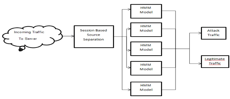
In the proposed HMM model as shown in Figure 1, the hidden states and observable variables considered are discrete because the CAIDA dataset contains only categorical distribution. The elements of HMM used for modelling are mentioned below
1. Number of hidden states representing attack and normal states.
Figure 1: Proposed Hidden Markov Model for Network Anomaly Detection of DDoS Attacks
3. Initial probabilities, which is a vector of size equal to number of states (1 ⋆ N) representing the probability that the sequence of the state will start with a given state. π is an array of length N representing the initial probability of being at state N.
4. Transitional probabilities, A is a two dimensional array. The state transition probability is a square matrix with size equal to the number of states (N ⋆ N) in which each element represents the transition probability from one state to another state.
5. Emission Probabilities, B is two a dimensional array. The observable probability is a non-square matrix, with dimensions equal to number of states by number of observables (N ⋆ M) where the probability that a given observable will be emitted by a given state.
Training:The primary objective is to determine the most appropriate model λ= (A, B, π) which can maximize the
conditional probabilities given the model parameters which are mentioned above. The most popular approach to solve the learning problem is Baum-Welch algorithm [2].
1. The model is trained separately using the normal and attack sessions from the CAIDA dataset.
2. The attributes are chosen using a feature selection tool such as WEKA which helps the model to learn its sessional characteristics.
3. The chosen attributes are TCP flags, Packet size, Source/Destination Port number,Source/Destination IP number.
4. The normalization process is primarily used to generate the initial, transition and emission probabilities. 5. The Forward-Backward algorithm is used to overcome the evaluation problems. The evaluation problem is to compute the probability of sequence of observations O which is produced by the model λ can be represented as P(O| λ) [2].
6. Re-estimation of initial, transition and emission probabilities of HMM as explained in section II. 7. The maximum likelihood is computed using Viterbi algorithm[2], Q = argmax[ δT(i) ]
8. The threshold is a minimum value which is selected among the fixed number of iterations. In this experiment the number of iterations considered is ten.
Testing:The primary objective of the HMM model is to predict the given session as normal or anomalous based on the
characteristics of the attributes considered at the time of training. The testing process is briefly explained below. 1. For a new session, the model calculates initial, transition and emission probabilities using Baum-Welch algorithm as explained above in section II.
2. The maximum likelihood is computed using Viterbi algorithm[2]
suspicious. 4.
V. PERFORMANCEEVALUATION
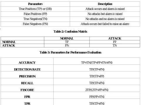
The model is evaluated in terms of their detection rate, false positive rate, precision, recall and F1-score as shown in Table 1, 2, 3 are explained below
Table 1: Parameters for Performance Estimation
Parameters Description
True Positives (TP) or (DR) Attack occurs and alarm is raised
False Positives (FP) No attacks but alarm is raised
True Negatives(TN) No attacks and no alarm is raised
False Negatives (FN) Attack occurs but failed to raise an alarm .
Table 2: Confusion Matrix
NORMAL ATTACK
NORMAL TP FP
ATTACK FN TN
Table 3: Parameters for Performance Evaluation
ACCURACY TP+TN/(TP+FP+TN+FN)
DETECTION RATE TP/(TP+FN)
PRECISION TP/(TP+FP)
RECALL TP/(TP+FN)
F1SCORE 2TP/(2TP+FP+FN)
FPR FP/(FP+TN)
TPR TP/(TP+FN)
ACCURACY:The proportion of the total number of correctly predicted attack and normal cases to the actual data set
size. It is not a good metric for comparison since the true negatives abound.
DETECTION RATE/RECALL:The proportion of correctly predicted attack cases to the actual size of the attack
class.
PRECISION:The proportion of correctly predicted attack cases relative to the predicted size of the attack class.
FALSE POSITIVE RATE: The rate at which normal connections are being flagged as attack.
VI. DATASETANDRESULT
In the proposed model, the HMM approach is used to evaluate the accuracy for the classification of CAIDA dataset.Experiments were conducted on both normal and attack dataset which were taken in ratio of 80% for training and 20% for testing. The resulting results have found to be satisfactory but addressing an attack situation in terms of making a system with zero false positive is still a challenge. The below Table 4,5 indicates the performance evaluation parameters used for training model using normal and attack dataset separately.
Table 4: Results For Normal Trained Dataset
Accuracy Detection Rate Precision Recall F1score FPR TPR
79.48 79.944 99.25 79.944 88.557 0.88235 0.79944
78.12 79.861 97.15 79.861 87.661 0.85075 0.79861
76 79.992 93.35 79.992 86.156 0.80121 0.79992
74.28 79.851 90.75 79.851 84.952 0.81498 0.79851
68.44 79.813 81.05 79.813 80.427 0.8081 0.79813
Table 5: Results ForAttack Trained Dataset
Accuracy Detection Rate Precision Recall F1score FPR TPR
79.14 98.077 80.225 98.077 88.257 0.96175 0.98077
76.07 94.093 79.651 94.093 86.272 0.95628 0.94093
75.3 92.995 79.554 92.995 85.751 0.95082 0.92995
75.41 92.171 80.072 92.171 85.696 0.91257 0.92171
69.71 84.066 79.275 84.066 81.6 0.87432 0.84066
VII. CONCLUSION
On the basis of analyzing session based behavioural approach of a TCP network traffic using a HMM model, a real-time DDoS attack detection and prevention system is realized. It has the below advantages
Session based traffic behaviour analyses helped to differentiate the attackers from the normal users
The model ensures that it achieves good detection rate and accuracy for CAIDA dataset
REFERENCES
[1] MonowarH.Bhuyan, H J.Kashyap, D K.Bhattacharyya and J K.Kalita, “Detecting Distributed Denial of Service Attacks: Methods, Tools and the FutureDirections”, The Computer Journal, Vol.15, pp. 23-35, 2013.
[2] Lawrence R.Rabiner, “A Tutorial on Hidden Markov Models and Selected Applications in Speech Recognition”,Proceedings of the IEEE,Vol.5, pp.12-15, 1989.
[3] S. Malliga, A. Tamilarasi, and M. Janani, “Filtering spoofed traffic at source end fordefending against DoS/DDoS attacks”,International Conference on Computing, Communication and Networking ,Vol.24, pp.1–5, 2008.
[4] Wang,Wei, Xiao-Hong Guan and Xiang-Liang Zhang,“Modelling the Program behaviors by Hidden Markov Models for intrusion detection system”, Proceedings of the IEEE International Conference on Machine Learning and Cybernetics, Vol.5, pp. 45-53, 2004.
[5]R Vijayasarathy, “A System Approachto Network Modelling for DoS Detection using a Naïve Bayesian Classifier”, Proceedings of IEEE on Network Security, Vol.54, pp.13-17, 2012.
[6]Robert Beverly, Arthur Berger and Young Hyun, “Understanding the Efficiencyof deployed internet source address validation filtering”, Proceedings of the SIGCOMM conference on Internet measurement, Vol.23, pp.321-34, 2009.
[7] Sung-Bae Cho and Hyuk-Jang Park, “Efficient anomaly detection byModelling privilege flows using Hidden Markov Model”,Journal of Computers networks and Security, Vol. 22, pp. 45-55, 2003.
[8] German FlorezLarrahondo, Susan M.Bridges and Rayford Vaughn, "Efficient modelling of discrete events for anomaly detection using Hidden Markov Models, " Proceedings of the 8th International Conference on the Information Security, Vol.78, pp. 506-514, 2005.
[9]Andr'e Ames, Fredrik Valeur, GiovanniVigna and Richard A. Kemmerer,“Using Hidden Markov Models to evaluate the risks of intrusions”,Proceedings of the Recent Advances in Intrusion Detection, Vol.74, pp. 145-164, 2006.