Analysis of Face Recognition Techniques with
Grayscale and Color Preprocessing
Dr.Gadiparthi.Manjunath
1, Daniel Abebe Negash
2, Nune Sreenivas
31Assistant Professor, Center of ITSC, AAiT, AAU, Addis Ababa, Ethiopia 2Head of the Department, Center of ITSC AAiT, AAU, Addis Ababa, Ethiopia
3Assistant Professor, SECE, AAiT, AAU, Addis Ababa, Ethiopia
ABSTRACT: Face recognition is an important aspect of biometric and is considered as low cost yet efficient method. The main concept of face recognition is extracting features, but it is easily affected by light condition and facial expression changed and other reasons. So before extracting features we can preprocess face images to improve the face recognition rate. In this work we introduce various preprocessing methods in face recognition and analyze the effect of recognition accuracy of various face recognition techniques processed with the preprocessing. Firstly, we present an overview of face recognition and its applications. LBP, Wavelet, Eigen features from face images are extracted after preprocessing and Neural Network and Nearest Neighbor classifier is used for recognition purpose. Results shows that preprocessing techniques combined with LBP and Neural Network Based Method produces best accuracy of 100% for 100 classes of face and 100 features.
KEYWORDS: Face recognition, wavelet transforms, DCT, Local binary pattern, KNN classifier, neural network
I. INTRODUCTION
Face recognition is a successful application in computer vision and also in the biometric system used to identify or verify a person from a digital image or a video frame from a video source [1]. Face recognition system can be generally classified in two groups. But within these groups, significant differences exist, depending on the application: image quality, background, exclusive image variability, availability user input[2] . There are a lot of applications of face recognition in different areas. It can be used in document control (passports and drivers license), in transactional authentication (credit cards and ATMs), in computer security (user access verification), in voter registration, in entertainment (video game, virtual reality or human-computer interaction) and in medical applications (emotions analysis and visual tracking) [3]. Face recognition is one of the few biometric methods that are highly accurate and low intrusive. Since the biometric data can be captured at a distance, it does not require active participation on the part of the subject. The infrastructure for its implementation is already widespread and inexpensive. Security cameras are currently common in airports, ATM machines and in any location with a security system.
Normally a face recognition algorithm can be divided in two functional modules: a face image detector, which finds the location of human face in cluttered scenes, and a face recognizer, which determines who that person is. The face detector has to decide between two image classes: “face” images and “non-face” images. In this project, only images with a unique human face have been considered. The face recognizer, on the other hand, involves extracting a features set from a 2D face image and matching it with the template stored in the database. Facial recognition systems should be able to automatically detect a face in an image, extracts its features and then recognize it, regardless of lighting and pose, which is a rather difficult task.
A face image is easily subjected to changes in viewpoint, illumination, and expression and so on. So the first issue is what features can be used to represent a face in order to be able to deal with possible changes and expression. Therefore, some preprocessing methods should be used in order to reduce these affections to some extent[1].
II. IMAGE PROCESSING METHODS
In this section some pre-processing methods are introduced to pre-process face images before extracting features.
A. Wavelet Transform
Wavelet transform technique is a new field in face recognition and it has an impact on some old and new disciplines. Compared with Fourier transform and Gabor transform, it can extract useful information effectively. Thus, it can solve some problems that Fourier transform can not resolve. Wavelet transform provides a powerful and versatile framework for image processing. It is widely used in the fields of image de-noising, compression, fusion, and so on. The changes of expressions in the sample images of an individual result in the differences of higher frequency band of the images. The basic functions of wavelet transform are obtained from a single prototype wavelet (or mother wavelet) by translation and dilation [4]:
Where a and b are both real numbers which quantify the scaling and translation operations. Substitute a and b with 2m and n×2m respectively, the basic functions become
The process of one-dimensional discrete wavelet transform and reconstruction a signal x (t) is defined as follows:
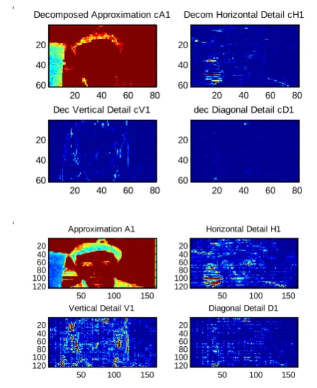
The two-dimensional wavelet transform is got by applying one-dimensional wavelet transform to the rows and columns of two-dimensional data An approximation image is derived from 1-level wavelet decomposition of an image and three detail images in horizontal, vertical and diagonal directions respectively. The approximation image is used for the next level of decomposition. Figure 1 is the process of decomposing an image, Figure2 is an image from ORL Face Database, Figure 3 is obtained after one-level wavelet transform.
B. Discrete Cosine Transform
When In the past two decades, there have been a variety of studies on the distributions of the discrete cosine transform (DCT) coefficients for images [5]. DCT decorrelates the image data, further each output can be ecoded separately, but there is no compression efficiency lost.
Figure (A) The process of decomposing an image
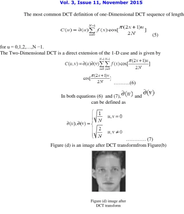
The most common DCT definition of one-Dimensional DCT sequence of length N is
(5)
for u = 0,1,2,…,N −1.
The Two-Dimensional DCT is a direct extension of the 1-D case and is given by
……….(6)
In both equations (6) and (7), and can be defined as
………… (7) Figure (d) is an image after DCT transformfrom Figure(b)
C. Color Normalization Methods
1)Intensity normalization:A well-known image intensity normalization method is applied here, and we can assume that, for the intensity of the lighting source is increased by a factor, in the image each RGB component of each pixel is scaled by the same factor. We can divide by the sum of the three color components to remove the effect.
2) Gray world normalization:Here we take an approach which is similar to the above normalization, but compensate for the effect of variations in the color of the light source. The RGB color components of an image can be caused by different colors of light cause to scale apart, by factors α, β and γ respectively.
3) Comprehensive color image normalization:
We apply an algorithm which is proposed by Finlayson [5], and it normalizes an image for variations in both lighting geometry and illumination color. The method involves the repetition of intensity normalization followed by grey world normalization (as described above), until the resulting image reaches a stable state.
4) Standard definition of hue: The hue of an image can be calculated by using the standard hue definition, such as each pixel is represented by a single scalar value H.
….. (9)
III. THEORETICAL BACKGROUND
A. PCA approach to Face Recognition
PCA is often used in many forms of data analysis, from neuroscience to computer graphics, being a simple non parametric method which extracts the relevant information from large data sets. PCA offer the solution of reducing a complex data set to a lower dimensional one with a good representation of the information for discriminative feature selection. The advantages of PCA were firstly explored by Turk and Pentland in their face recognition method [6]. For that, a training face image database is needed. The training face images set selection is crucial for representative enough for the given classification problem.
When we apply PCA, the most significant eigenvectors are extracted from the training database, and they define a lower dimensional subspace. They are also known as “the eigenfaces” [6] due to their graphical representation. After computing the eigenfaces, any face image is represented by a feature vector in the subspace determined by the eigenfaces. A short summary of the algorithm [2] is presented below:
For a grey level N × N image, we consider it as a N2 one-dimensional vector. Let X be a matrix of S columns and N2 rows, where S represents the number of training images, which can be used to represent the entire training set of face images.
….. (10)
The goal of PCA is to derive another matrix P matrix which will describe a linear transformation of every column in X
(every training face) in the eigenfaces subspace, in the form: W=PX, where W are the projections of the training facial images on the subspace described by the eigenfaces. The rows of P matrix represent the principal components and they are orthonormal.
The computation of the matrix P requires the following: • Find the mean face vector M, as in (2), where
Xi (i=1,2,…,S) represents the ith column of X:
……… (11) • Subtract the mean face M from each training
face Xi:
……….. (12) • Compute the covariance matrix CA, where A=
[H1, H2... HS]:
For every image, a projection on the subspace will be extracted. The projection of the test image is compared with each training projection in all the classical approaches on visible spectrum. The decision process is based on a classifier in the projections space and it returns the identity of a person. In the basic approach of Turk and Pentland [6], a simple minimum Euclidian distance classifier is used.
B. Local Binary Pattern
The LBP operator [7] is one of the best performing texture descriptors and it has been widely used in various applications. Is a key advantage, computational efficiency makes it suitable for demanding image analysis tasks
(i). LBP Operator:
The original LBP introduced by Ojala is a powerful texture descriptor with computational simplicity in the scale of gray and has been successfully used in visual inspection and image retrieval, etc. It analyses the features of the fixed window in method of structure first, and then utilizes statistical methods to extract the whole feature. The pixels are labelled by the operator by threshold. The result as a binary string or a decimal number .Then the histogram of the labels can be used as a texture descriptor [8]. The LBP produces 2^8=256 texture patterns. The output value of LBP operator can be defined as follows:
…………. (15)
Where R is radius, P is the number of pixels in the circle,pi is the value of the neighboring pixel, pc is the value of the center pixel and
………. (16)
When (P, R) is (8, 1), it is a standard LBP. The detailed description of LBP operator can be found in Fig. 1. The LBP was first used in the area of face recognition by Ahonen [2]. For avoiding the localization, Ahonen utilized he histogram of LBP to improve the spatial relation among the local patterns [6-7]. Fig. 2 gives the LBP and histogram of two different facial images, comparing (a) with (b), we found that the LBP encoding in Fig. 2 (b) has the visual characteristics from original such as glasses. This proved that the LBP feature is an excellent measure of the special structure of the local image texture, and can represent the microstructures including the bright or dark spots, the edges. The distribution of these features is described with the histogram. Abscissa of histogram presents the greyscale and ordinate presents the number of pixels.
Figure1.Basic LBP operator
(ii). The histogram features:
The histogram of encoding describes the texture and Structural characteristics through distribution of abscissa, the definition as follows:
… (17) and
……… (18)
The histogram contains the distribution of the local micro features, such as facial contour, stability area of face. As shown in the Fig. 2, transverse axis of histogram represents the greyscale and vertical y-axis represents the number of pixels which greyscale is x.
C. KNN Classifier
K-NN is a supervised classification method in a given feature space – in our case, the eigenfaces space extracted with PCA. To build the k-NN classifier, one simply needs to define the number of classes C, to form a labelled training set of Ntrn samples in the feature space, with class labels yi=1..C, and to consider the labelled samples in the training set as known prototypes of the C classes. Furthermore, a distance norm d in the feature space must be chosen for the data classification (e.g. the Euclidean distance). Suppose that a vector W from the feature space must be classified in one of the C classes. By k-NN, W is as its k nearest neighbours in the sense of the distance norm chosen, being classified as the class which is mostly common within them [4].
The algorithm needs to follow the steps:
• Compute the distances d(W,Wt,j) for each prototype (denoted by Wt,j, j=1,2,…,Ntrn) from the training set.
• Sort the distances d(W,Wt,j), j=1..Ntm, increasingly, and keep the labels of the first k prototypes (found at the first
k smallest distances from W): {y1’, y2’,…,yk’}.
• Assign to W the yl’ label, most frequent from the class sort array {y1’, y2’,…,yk’}.
IV. HELPFUL HINTS
In this paper, we use the ORL database of faces which is usually used in face recognition. There are forty persons in the database, and for each person they are ten images. Within the database some images were taken at different times, with different lighting and facial expressions. For the pre-processing we use image of the real faces. The figure below shows the output of pre-processing methods.
Figure (d) Figure (e)
Figure (f) Figure (g)
dct color map
color normalized image
Image after recovery from DCT
Hue image Figure(c). Image preprocessing using extended pseudo color of
Db2 wavelet transform
Approximation A1
50 100 150
20 40 60 80 100 120
Horizontal Detail H1
50 100 150
20 40 60 80 100 120
Vertical Detail V1
50 100 150
20 40 60 80 100 120
Diagonal Detail D1
50 100 150
20 40 60 80 100 120
Figure (b). Image preprocessing using Db2 Wavelet transform
Decomposed Approximation cA1
20 40 60 80
20
40
60
Decom Horizontal Detail cH1
20 40 60 80
20
40
60
Dec Vertical Detail cV1
20 40 60 80
20
40
60
dec Diagonal Detail cD1
20 40 60 80
20
40
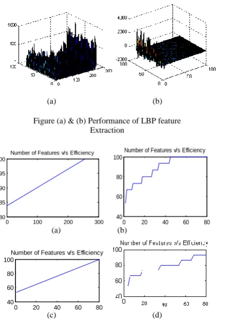
The above Figure shows the performance of face recognition with various methods. Fig(c) & (d) is the performance of LBP feature extraction with KNN classifier and as well as neural network .Fig (e) &(f) ) is the performance of Eigen feature extraction with KNN classifier and as well as neural network.
V. CONCLUSION
In this paper, we shortly introduce some image preprocessing methods used in face recognition and analyze the effect of the same in face recognition. The performance of PCA method is highly dependent on the image capture conditions and it is easily affected by Variations in lighting conditions, differences in pose, and image quality and so on, so it is necessary to preprocess these face images to improve the face recognition rate. In this paper we use different methods of face recognitions like LBP, KNN classifier, neural network. The performance of face recognition is by comparing methods with one another. Most of the time, we often combine two or more preprocessing methods so as to achieve a better result.
REFERENCES
[1] Zhang Haiyang “Image Preprocessing Methods in Face Recognition” College of the Globe Science and engineering, Suzhou University Suzhou, Anhui province, China,234000 978-1-4244-6554-5/11/$26.00 ©2011 IEEE
[2] Xiaoyang Tana, Songcan Chena, Zhi-Hua Zhou, Fuyan Zhang, 2006. "Face recognition from a single image per person: A survey, Pattern Recognition", Vol. 39, 2006, pp. 1725 – 1745.
[3] W. Zhao, R. Chellappa, A. Rosenfeld, P.J. Phillips, Face Recognition: A Literature Survey, ACM Computing Surveys, 2003, pp. 399-458. [4] Yugang Jiang, Ping Guo. “Face Recognition by Combining Wavelet Transform and k-Nearest Neighbor.” Journal of Communication and
Computer, Vol.2, Sep.2005.
(a) (b)
(c) (d)
0 100 200 300
80 85 90 95 100
Number of Features v/s Efficiency
0 20 40 60 80
40 60 80 100
Number of Features v/s Efficiency
0 20 40 60 80
40 60 80 100
Number of Features v/s Efficiency
(a) (b)
Figure (a) & (b) Performance of LBP feature Extraction
[5] R. Samadani, A. Sundararajan, and A. Said, “Deringing and deblocking DCT compression artifacts with efficient shifted transforms,” in Proceedings of the International Conference on Image Processing (ICIP), 2004
[6] T. Ojala, M. Pietikainen, and D. Harwood, “A comparative study of texture measure swith classification based on feature distributions”, Pattern Recognition, vol. 29, pp. 51-59,1996.
[7] T. Ahonen, A. Hadid, and M.Pietikainen, “Face Recognition with Local Binary Patterns”,Proc. 8th European Conference on Computer Vision(ECCV 2004), Springer Press, May 2004, pp. 469-481.
[8] T. Ahonen, and A. Hadid, “Face Recognition with Local Binary Patterns: Application on Face Recognition”,Proc. IEEE Transactions on Pattern Analysis and Machine Intelligence ,IEEE Press,2006,pp.
2037-2041.
[9] A. Pentland, B. Moghaddam, and T. Starner, “View-Based and modular eigenspaces for face recognition,” Proc. IEEE CS Conf. Computer Vision and Pattern Recognition, pp. 84-91, 1994.