Division 4
LANDFORM- TO MICROSTRUCTURAL-SCALE VISUALIZATION
AND ANALYSIS OF FAULT ZONES: USE OF UNMANNED AERIAL
VEHICLES AND STRUCTURE FROM MOTION FOR TOPOGRAPHIC
ANALYSIS
Cline, M. Logan1, K.M. Cline2, C. Cinkilic3, M. Rosenmeier4, D. Raszewski5, D. Eysenbach6.
1
Director of Geosciences, RIZZO Associates, United States
2
Chief Geologist, RIZZO Associates, United States
3
Senior Engineer, RIZZO Associates, United States
4
Director of Hydrogeology, RIZZO Associates, United States
5
Senior Geologist, RIZZO Associates, United States
6
Planning and Environmental Coordinator: Bureau of Land Management, United States
ABSTRACT
Fault zone characterization for seismic hazard analysis requires quantitative geomorphic analyses aimed at constraining the geometry and rates of fault deformation occurring at or near the surface. Over the past decade, high-resolution topographic data from laser altimetry (i.e. lidar) have become the gold standard for these geomorphic analyses; however, lidar acquisition can be cost prohibitive, particularly for small projects, and airborne lidar platforms cannot typically be deployed on short notice, or access complex or otherwise restrictive terrain. Recent advances in computational power and computer vision technology have enabled rapid construction of true three-dimensional (3D) topographic models from dense photo datasets via structure from motion multi-view stereo photogrammetry, which is a low-cost alternative to developing extremely high-resolution digital topographic models. The availability of low-cost, unmanned aerial vehicles provides an ideal platform for dense photo acquisition, and facilitates production of SFM-MVS-based topographic datasets that dramatically exceed the resolution of airborne lidar. Furthermore, the flexibility afforded by cameras deployed on small UAVs reduces logistical complications and allows for scale-independent mapping.
We present early results from the 2014 M 6.0 South Napa Valley Earthquake surface rupture in the U.S. to evaluate the efficacy of SFM-MVS for detailed fault characterization. Our SFM-MVS results demonstrate that ability to detect extremely subtle, small-scale deformation features standard airborne lidar cannot resolve. SFM-MVS data are compared with terrestrial laser scanning data for validation. The small-scale deformation features have considerable implications for seismic source modelling, particular for site-specific, probabilistic fault displacement hazard analyses.
BACKGROUND
Advances in SFM-MVS and UAV
imagery; however, unlike stereo imagery SFM-MVS does not require controlled spacing of images and precise calibrations of lenses and ground control for model development. Instead, SFM-MVS relies on unordered, densely-acquired photo datasets to produce true 3D digital models of objects or landforms that can be scaled accordingly.
Parallel advances in semi-autonomous flights of small, unmanned aerial vehicles (UAVs) have facilitated the rapid expansion of SFM-MVS-based 3D digital models. Combined, these advances facilitate low cost and rapid data production with remarkably high resolution, high 3D geometric precision, and the potential for high spatial accuracy. Small UAVs are regularly fitted with “smart” flight capabilities that enable them to fly in most conditions, even in windy, dusty, and damp conditions using semi-autonomous piloting. UAVs are able collect data in areas where manned aerial vehicles cannot access, including inside of structures and mines. Their ability to access precarious locations removes humans from harm’s way when investigating unsafe site conditions.
Combining UAV platforms with SFM-MVS, large areas (hectares) can be mapped within minutes. This technological merger has created wide-ranging applications for SFM-MVS that span virtually every field that utilizes 3D or orthorectified two dimensional (2D) visualization for analytical or visualization purposes. RIZZO employs these technologies for many of its projects, and RIZZO scientists regularly collaborate with researchers from the US Geological Survey optimize workflows for cutting-edge applications.
SFM-MVS is a scale-independent algorithm that relies on recovering camera parameters (e.g. 3D position, camera orientation, and lens distortion) from multiple photos to reconstruct 3D scene structure (Snavely et al., 2008). At its core, SFM-MVS model parameters are derived internally, solely from the images; however, modern techniques and digital data allow for optimization based on the image metadata (e.g. exchangeable image files [EXIF]). The initial steps for the image-based modeling involve the accurate identification of keypoints, which involves object identification that relies on unique image attributes (Snavely, 2008). Object recognition is scale independent; it compares keypoints between image pairs to find those with common attributes. The process is iterative, which allows for expunging erroneous keypoints that are identified during early iterations. Keypoints shared between image pairs are continually added until the orientations of camera positions associated with each photo are iteratively calculated and optimized based on error minimization routines (i.e. Snavely, 2008; Westoby, 2012). Keypoints are mosaicked in 3D computational space, which facilitates the 3D construction of the relative scene geometry. To achieve absolute scaling and/or georeferencing either ground control points (GCPs) or camera-position global positioning system (GPS) is necessary. Typically, GCPs provide robust quality control on image geometry; however, in the event that GCPs cannot be placed due to hazardous condition or other logistical reasons on-board real-time kinematic (RTK) GPS can be used so that the camera can accurately geotag camera image positions. Alternatively, positional accuracy can be performed during the post-processing (as in this study) using existing georeferenced datasets. For a thorough description of the full SFM-MVS process, refer to Snavely et al., (2008), Granshaw (1980).
The dataset resulting from the SFM-MVS process is constellation of points (typically millions to billions) in x, y, z, space, known as a point cloud. The points have additional attributes such as color (RGB) values that can be used to render detailed, 3D textural models.
Tectonic geomorphology
engineering purposes, as small-scale processes are those which define the broader-scale, and thus there is opportunity for mitigating hazards by recognizing and addressing the smaller-scale processes.
In paleoseimology and tectonic geomorphology, small displacements (<1 m) of the surface have historically gone unrecognized unless pronounced, discrete ruptures occur. Even a geologically recent fault surface rupture leaves a transient surface expression, and its topographic persistence is limited by climate, material strength of the deformed soil or rock, and its position on the landscape (i.e. exposure to erosion). Over longer timescales the fault surface rupture may diffuse to the point it is nearly undetectable, but the broader landscape often archives deformation by controlling the topographic relief, or the shape of a river’s longitudinal profile (e.g. Wobus et al., 2006). Over the past decade, the increased spatial coverage of digital topography from photogrammetric and lidar surveys have dramatically enhanced our ability to detect these features past decade or so because they can resolve the shape of the earth’s surface at very fine spatial scales; however, only a small fraction of the globe has lidar coverage, and the cost of acquiring new data can be cost-prohibitive. Furthermore, the cost of lidar acquisition makes temporal change detection beyond the reach of most projects.
GENERAL APPROACH
Data acquisition strategies vary based on the desired data format and site conditions. The following discussion focusses on the production of topographic datasets used in geomorphic and geological analyses, which commonly entails the production of a bare-earth digital elevation model (DEM) (i.e. a 2.5D model of the ground surface, free of vegetation). We also provide a brief discussion on some of the inherent challenges and error mitigation strategies.
Flight planning considerations
Standard UAV-based SFM-MVS mission planning begins by defining the key area of interest and then designing the most appropriate gridded (or otherwise) flight path and altitude to achieve the desired resolution. There are numerous softwares and mobile apps that optimize these parameters. These are fundamental because the quality of the 3D model (resolution and accuracy) is a function of camera overlap and image resolution. Resolution of the final model is a function of the camera’s pixel resolution, image sensor, and the camera’s distance from the target resolution, whereas image overlap is controlled by the flight path grid pattern, flight velocity, and digital camera’s write speed. Achieving optimal overlap is imperative because every point that is modeled in 3D space (i.e. those that make up the point cloud) requires that at least two camera positions that can see it. In open terrain, this is a trivial matter, but on terrain with complex topography, overhangs, and vegetation, flight planning strategies are more rigorous. As a general rule, is imperative that images overlap >75% for accurate surface modeling in open terrain, but in complex terrain with high vegetation density, greater image overlap is necessary.
Topographic complexity leads to variability in the fidelity of features on the ground. In deeper valley, for example, where the camera position may be hundreds of meters above the ground surface, but only tens of meters above the peaks and ridges. As a result, the model would result in low fidelity of valley features and high fidelity of peaks and ridges. Furthermore, objects on the edges of the camera’s field of view will often be imaged in lower resolution.
Dealing with vegetation and other image-obscuring conditions
and fly either within the canopy or just above the canopy for the second pass. This will help to image the ground surface through gaps in vegetation. Sub canopy flights are ideal but require a highly trained pilot. In additional, hand-held and pole-mounted images can be used within the canopy to image the ground surface. Figure 1 shows an idealized example of camera positioning for image acquisition that allows for full feature mapping of vegetation and ground surfaces.
In Figure 1, camera positions A and B are able to clearly see the vegetation tops, but due to the limited canopy penetration of the images and shadowing of the ground surface, the camera positions do not allow for imaging the ground. Camera positions C and D, however, are able to clearly see the ground using down-facing and oblique camera angles.
.
Figure 1
Idealized camera positions to capture vegetation and ground surface geometries.
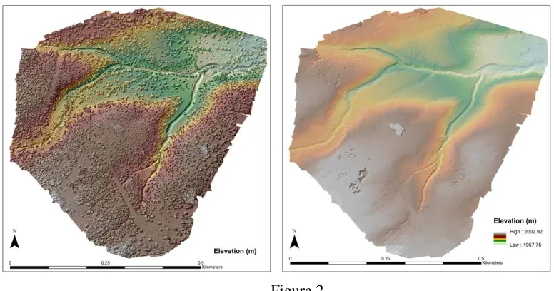
An inherent strength of SFM-MVS is that it does not require that photos be captured from the same x,y plane, so in the event that canopies block overhead views but allow understory photo acquisition, lower or more oblique photos can be used to infill the photos to define the ground surface. This arrangement facilitates the production of bare-earth DEMs, but may not always be feasible when canopy density is excessive. Figure 2 shows an example one of our research sites in NM, which shows a “full feature” (left) and a bare-earth (right) DEM produced from the same SFM-MVS point cloud.
Figure 2
Example of vegetation removal from SFM-MVS data is shown. The left side shows a full-feature hillshade with an elevation-colored overlay. The right side shows the same dataset, after classifying the
Mitigating inherent SFM-MVS errors during data acquisition
Common practice has been to collect photos that are nadir-oriented, parallel-axis photographs to construct DEMs along a single elevation plane using a gridded approach. Contrary to this systematic and seemingly logical approach, research has shown the acquisition strategy results in vertically distorted DEMs, whereby broad-scale deformation of the surface is expressed as doming (e.g. Wackrow and Chandler, 2008; Wackrow and Chandler, 2011). Traditional stereo-photogrammetry does not suffer from these issues to the same extent as the SFM-MVS procedure because of rigorous processing, dense networks of ground control points (GCPs), and the use of camera lenses with negligible radial distortion (e.g. James and Robson, 2014). Now that consumer and commercial-grade UAVs and digital cameras are more accessible, and the fact that, for many users, SFM-MVS softwares are “black boxes” systematic errors are increasingly prevalent. This is particularly troubling if the errors go unnoticed, which result in erroneous DEMs, and when used in calculations, ensures and propagates errors. In the worst case, this places infrastructure or human life at risk if, for example, rainfall runoff models or slope stability calculations are based on flawed DEMs. It is a particular significant issue for surface tectonic deformation modelling. A final DEM showing warping from the processing could result in the incorrect interpretation of surface deformation (e.g. uplift or subsidence zones). The core of the issues is the inherent radial distortion of most camera lenses, and the erroneous correction of the distortion that occurs in most SFM-MVS softwares, which is exacerbated by the parallel-axis alignment of camera locations and orientations (e.g. Eltner and Schneider, 2015; James and Robson, 2014; Wackrow, 2008; Wackrow and Chandler, 2011). Fortunately, research on this issue has developed recommendations to mitigate the error source (e.g. James and Robson, 2014; Fondstad et al., 2013; James and Robson, 2012; Wackrow and Chandler, 2011).
To create the most accurate DEM we apply the guidelines described in James and Robson (2014), as well as our own methods that are optimized for geomorphic applications. These are summarized in the bullets below:
• Convergent image pairs should be used to supplement the standard, parallel axis photo pairing. • Orbital flight paths that take oblique images with a convergent orientation should be used to
supplement the standard, gridded, parallel-axis photo pairing.
• Off-nadir images should always be used when following a traditional, gridded flight path. • Photos should ensure adequate overlap (minimum of 75%) in open areas (e.g. open fields), and
increase overlapping in more complex terrain (e.g. high topographic ruggedness or high vegetation cover).
• Image datasets are supplemented with images from multiple elevations, orientations, and obiquities.
Post-processing image data
successfully differentiate, for example, a boulder strewn landscape from a shrubby landscape. Therefore the post-processing of point clouds could have profound effects on rainfall-runoff modeling, or other analyses requiring detailed characterization of the ground surface.
DEM and Point Cloud Production
The vast majority of tools for analyzing topographic data rely on DEMs, which can be thought of as a 2.5 dimensional (2.5D) representation of the earth’s topography. It is 2.5 D because each discrete x,y, coordinate can only have a single z (i.e. elevation) value. On the contrary, a point cloud can be defined by multiple, discrete z values at any single x,y coordinate position. For example, a bridge and the river or water beneath it may be defined by no less than three z values at each x,y, coordinate: one for the upper deck, one for the lower deck, and one for the ground or water. A DEM will can only define that same bride with a single point, which represents the elevation of the upper deck. DEMs are simple raster (i.e. gridded) datasets that form the basis for efficient calculations and analyses. For geoscience applications that focus on the earth’s surface, a bare-earth DEM is adequate for most analyses; bare-earth DEMs are also adequate for cut-fill calculations, flood modeling, and earth works applications in engineering.
CASE STUDY RESULTS
The 2014 M6.0 South Napa Earthquake produced a small coseismic surface rupture along part of its trace, and following the event, spatially complex but surprisingly large post-seismic slip (i.e. afterslip) has been occurring (e.g. DeLong et al., 2015; Leinkamper et al., 2016; Delong et al., 2016). The South Napa Earthquake rupture provides a unique opportunity to investigate relatively small rupture and afterslip. Its small surface morphological features provide an excellent opportunity to evaluate the efficacy of SFM-MVS, and the presence of other datasets (multiple airborne lidar flights and terrestrial lidar scan [TLS] surveys) allow for data validation. Furthermore, the geographic region where the earthquake rupture occurred is ideal for investigating small surface ruptures because of the ubiquity of cultural features that record fine-scale deformation, such as fence lines and grape vine rows.
Earthquake scaling relationships (e.g. Leonard et al., 2010; Wells and Coppersmith, 1994) demonstrate that earthquakes ≤M 6.0 rarely exhibit surface rupture. It is therefore unsurprising that the M 6.0 South Napa event lacked significant rupture. Post-event reconnaissance mapping suggested maximum coseismic rupture, plus immediate after-slip ranged from 0.22 m to 0.29 m (first 2.5 days, Delong et al., 2015). What was unique, however, was the well-documented after-slip on faults (Leinkamper et al., 2016). Many ruptures increased ~20 cm during the two months following the earthquake (Delong et al., 2016). Our study focussed on the detection limits of UAV-based SFM-MVS DEM production to detect additional afterslip, and to recognize evidence for complex strain partitioning across small spatial scales. Details of change detection using terrestrial and airborne lidar and interferometric synthetic aperture radar (InSAR) following the South Napa Earthquake can be found in Delong et al., (2015; 2016).
Figure 3
2016 SFM-MVS DEM (left) and 2014 Airborne lidar merged with TLS (right)
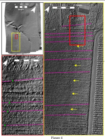
We performed the data collection during the early wet season so grass cover was relatively tall and dense. As a result, we had no expectation of resolving small-scale (10 cm or less) en echelon rupture traces that had been observed when the grass was dormant (see Delong et al., 2015); However, the DEM clearly resolved fine-scale slope breaks associated with long-term fault deformation, small-scale slope failures, and upon close examination, breaks in fence lines and grape fine rows. Figure 4 shows the zoomed view of the fault rupture, which displaced a steel fence and grape vine rows.
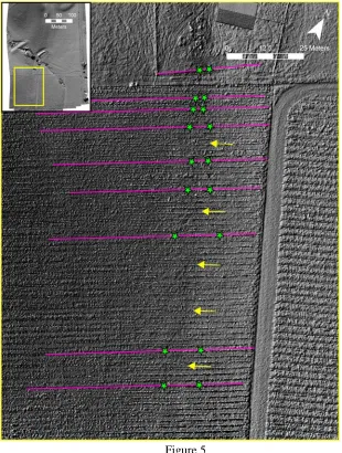
Displacement measurements exploited the many cultural features that cover the landscape, including grape vine rows and fence lines. The features are constructed along straight lines, which is common practice for the region. Offset measurements were made at several locations to the east and west of the mapped fault trace. The measurements we made by simply projecting the straight vine row lines, and then measuring the deflection of the current vine row positon for the projection of the vine row. The orientation of each measurement was consistent with the mapped fault trace. The displacement was relatively consistent throughout the vine rows and fence, suggesting roughly 40 m of surface displacement. We also measured width of the deformation zone. We simply utilized the deflection points of the fence and vine rows to determine this. Figure 5 shows the morphological, long-term fault trace and the fault deformation band width.
Figure 4
Multiple zoom levels showing various indicators of tectonic deformation. Upper left: overview of the SFM-MVS hillshade; right image: projected vine row lines (magenta lines), and the subtle slope break
associated with long-term fault deformation (yellow arrows); lower right: zoomed image showing the displacement and peak deflection of vine rows (green stars).
additional scan covering this region in greater detail and further to the south would likely provide the necessary data to do more detailed analysis.
Figure 5
Fault zone width is indicated by the green stars. Note the subtle slope break (yellow arrows) falls within the fault zone, further supporting the slope breaks long-term tectonic origin.
CONCLUSIONS AND IMPLICATIONS FOR SEISMIC HAZARD ANALYSIS
Critical infrastructure often requires site-specific seismic hazard analyses and where there are active faults (or recently active), detailed tectonic geomorphic analyses can provide meaningful constraints on seismic source models. Our study validates the data quality provided by SFM-MVS by comparing it with a merged airborne lidar and TLS dataset. Furthermore, it highlights the ability to constrain not only the location, but also to recognize complex faulting patterns at the surface more than two years after a relatively small event.
time, there is no established paleoseismic method for evaluating afterslip in trenches. A long-term proposition is to develop an afterslip database for instrumental events. Perhaps this will lead to the recognition of key fault attributes that lead to considerable afterslip. It is also important to recognize that strain partitioning along a single fault may transition from simple, single trace faulting to more disperse faulting, and the transition can occur over relatively short wavelengths. In the case of our study, the maximum change in deformation zone-width takes place over 40-50 m along fault strike. The surface expression suggests that the deformation band may be spread over 10 m or more, and thus paleoseismic investigations should account for this possibility.
SFM-MVS provides a low-cost alternative to airborne lidar. While it may lack the ability to penetrate dense vegetation canopies like lidar can, it provides greater resolution, and comparable accuracy and precision, rivalling that of TLS, particularly when coregistered with existing point clouds, or when an abundance of ground control points can be used for georeferencing.
REFERENCES
[1] Hudnut, Kenneth W., Brocher, T.M., Prentice, C.S., Boatwright, J., Brooks, B.A., Aagaard, B.T., Blair, J.L., Fletcher, J., Erdem, J.E., Wicks, C.W. and Murray, J.R., "Key recovery factors for the August 24, 2014, South Napa earthquake." US Geol. Surv. Open-File Rept 1249 (2014): 51.
[2] DeLong, Stephen B., Donnellan, A., Ponti, D.J., Rubin, R.S., Lienkaemper, J.J., Prentice, C.S., Dawson, T.E., Seitz, G., Schwartz, D.P., Hudnut, K.W. and Rosa, C. "Tearing the terroir: Details and implications of surface rupture and deformation from the 24 August 2014 M6. 0 South Napa earthquake, California." Earth and Space Science 3.10 (2016): 416-430.
[3] DeLong, Stephen B., Lienkaemper, J. J., Pickering, A. J., & Avdievitch, N. N. "Rates and patterns of surface deformation from laser scanning following the South Napa earthquake, California." Geosphere 11.6 (2015).
[4] DeLong, Stephen B., Prentice, C.S., Hilley, G.E. and Ebert, Y. "Multitemporal ALSM change detection, sediment delivery, and process mapping at an active earthflow." Earth Surface Processes and Landforms 37.3 (2012): 262-272.
[5] James, M. R., and Stuart Robson. "Straightforward reconstruction of 3D surfaces and topography with a camera: Accuracy and geoscience application." Journal of Geophysical Research: Earth Surface 117.F3 (2012).
[6] James, Mike R., and Stuart Robson. "Mitigating systematic error in topographic models derived from UAV and ground‐based image networks." Earth Surface Processes and Landforms 39.10 (2014): 1413-1420.
[7] Lienkaemper, James J., Stephen B. DeLong, Carolyn J. Domrose, and Carla M. Rosa. "Afterslip behavior following the 2014 M 6.0 South Napa earthquake with implications for afterslip forecasting on other seismogenic faults." Seismological Research Letters (2016).
[8] Snavely, Noah, Steven M. Seitz, and Richard Szeliski. "Modeling the world from internet photo collections." International Journal of Computer Vision 80.2 (2008): 189-210.
[9] Tarolli, Paolo, J. Ramon Arrowsmith, and Enrique R. Vivoni. "Understanding earth surface processes from remotely sensed digital terrain models." Geomorphology 113.1 (2009): 1-3.
[10] Wackrow, Rene, and Jim H. Chandler. "A convergent image configuration for DEM extraction that minimises the systematic effects caused by an inaccurate lens model." The Photogrammetric Record 23.121 (2008): 6-18.
[11] Wackrow, Rene, and Jim H. Chandler. "Minimising systematic error surfaces in digital elevation models using oblique convergent imagery." The Photogrammetric Record 26.133 (2011): 16-31. [12] Westoby, M. J., et al. "‘Structure-from-Motion’photogrammetry: A low-cost, effective tool for
geoscience applications." Geomorphology 179 (2012): 300-314.