BREAKAGE ON THE DOWNSTREAM
TOPOGRAPHY: MORPHOLOGICAL
EVOLUTION OF MOUNDS AND A
FURROW
Magua Amos Ng’ang’a (M.Sc.)
Reg. No. I84/25459/2011
A thesis submitted in partial fullfilment for the Degree of
Doctor of Philosophy (Ph.D) in Applied Mathematics in
the School of Pure and Applied Sciences of
Kenyatta University
Declaration
This thesis is my original work and has not been presented for a degree award in any other university or for any other award.
Amos Ng’ang’a Magua
Signature... Date...
This thesis has been submitted for examination with our approval as university supervisors.
Dr. David Malonza
Signature... Date... Department of Mathematics
Kenyatta University
Dr. Mark Kimathi
Signature... Date... Department of Mathematics
Technical University of Kenya
Dr. Isaac Chepkwony
Signature... Date... Department of Mathematics
Dedication
Acknowledgements
My sincere thanks, glory and honour goes to the Almighty God for his unfailing provision, protection and sustenance throughout the study period.
I am greatly indebted to my supervisors, Dr. Mark Kimathi who has tirelessly inspired me to undertake this dissertation. His timely encouragement, friendship and support have not only made the completion of this dissertation possible but has left an impression which will continue to influence my work. Dr. David Malonza and Dr. Isaac Chepkwony who apart from being my lecturers and giving me good background in modelling made enthusiastic participation, valuable suggestions and continuous encouragement during the dissertation.
I specially thank Prof. Francis Gatheri for reading my work and giving valuable suggestions.
Acknowledgment is also extended to Dr. Benard Kivunge the Chairman Math-ematics department for his warm friendship and his continuous encouragement during the dissertation.
I extend my gratitude to Dr. Kube Ananda and Mr. Fidelis Magero for their invaluable assistance in inducting me to the latex typesetting system.
I sincerely thank the Dean’s office for the financial support i received through the dean’s research grant which boosted and enhanced the undertaking of this dissertation. Special thanks also to AMMSI for the sponsorship to the First Kenyatta University Mathematics Conference.
Declaration ii
Dedication iii
Acknowledgement iv
Table of Contents v
List of Figures vii
Nomenclature ix
Abstract xi
1 INTRODUCTION 1
1.1 Definition of terms . . . 1
1.2 Background Information . . . 4
1.3 Statement of the problem . . . 6
1.4 Hypothesis . . . 8
1.5 Objectives . . . 8
1.5.1 General objective . . . 8
1.5.2 Specific objectives . . . 8
1.6 Significance of the study . . . 9
1.7 Outline of the thesis . . . 10
2 LITERATURE REVIEW 13 3 THE GOVERNING EQUATIONS 24 3.1 Derivation of Shallow Water equations . . . 24
3.1.1 The conservation of Mass . . . 25
3.1.2 The Conservation of Momentum . . . 26
3.1.3 Boundary conditions . . . 28
3.1.4 Boundary Layer Theory . . . 29
3.1.5 Hydrostatic Pressure . . . 30
3.1.6 Horizontal Mean Velocity . . . 31
3.1.7 The simplified Momentum Equations . . . 32
3.1.8 Depth Averaging . . . 32
3.1.9 The Final form of Shallow Water Conservation Equations (Hydrodynamics Equations) . . . 35
3.1.10 Bed-updating Equation . . . 36
3.1.11 The Final form of the Governing Equations (Morphody-namic Equations) . . . 39
3.1.12 Non-dimensionalization . . . 40
4 NUMERICAL METHODS 44 4.1 C-Formulation . . . 46
4.1.1 Steady Approach . . . 47
4.1.2 Unsteady Approach . . . 47
4.2 Eigenvalues for the Jacobian of the flux matrix, F . . . 50
4.3 Eigenvalues for the Jacobian of the flux Matrix, G . . . 54
4.4 Relaxed System of the C-Formulation . . . 58
4.5 Spatial Discretization . . . 60
4.6 Time Discretization . . . 64
4.7 The initial and boundary conditions . . . 66
4.7.1 Specification of the initial conditions . . . 66
4.7.2 Specification of the Boundary Conditions . . . 68
4.7.3 Specification of the flow variables at the wall in the case of the furrow . . . 69
4.7.4 Specification of the flow variables at the wall in the case of the mounds . . . 71
5 RESULTS AND DISCUSSION 73 5.1 Morphological evolution of a furrow located downstream of the dam breach. . . 73
5.2 Morphological evolution of two mounds located downstream of the dam breach . . . 83
5.3 Conclusion . . . 92
5.4 Recommendations for further research . . . 97
References 98 A Summary of Equations 103 A.1 Formula for solving the cubic functions . . . 103
1.1 Chesbro dam and reservoir located in Llagas in Northern California 5 1.2 Flooding in Glashutte after the dam break in 12th August 2002 6
3.1 The Free surface Flow . . . 25
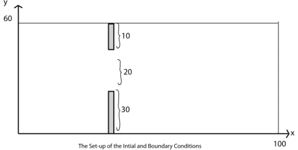
4.1 The set-up of the initial and Boundary Conditions . . . 66
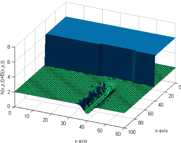
5.1 The Initial Set-up of the topography and the dam shortly before the dam break. . . 74
5.2 Glashutte Embankment dam overtopping on 12th August 2002 shortly before dam failure. . . 75
5.3 Water depth rise after the partial dam break. . . 75
5.4 The Depth contours and velocity vector plots for the partial dam -break flow. . . 77
5.5 The Depth contours and velocity vector plots for the partial dam -break flow zoomed to show the progress of entrainment from x= 55 . . . 77
5.6 Failure of the 207 feet high Auburn Cofferdam on the American river on February 18 1986. . . 78
5.7 The velocity vector contours and their corresponding magnitudes. 78 5.8 Aerial view of the furrow at T=2 for a dam break scenario without the entrainment. . . 79
5.9 Aerial view of the furrow at the period T=2 for the dam break scenario with entrainment. . . 80
5.10 Aerial views of the topography before the dam break and after the dam break for the dam break scenario with the entrainment. 80 5.11 Aerial view of the furrow at periods T=1.5, T=3 and T=4 for a dam break scenario with the entrainment. . . 81
5.12 The comparison of the furrow profiles in the dam break scenario with entrainment and without the entrainment. . . 82
5.13 Dam break flow scenario with entrainment. . . 85
5.14 Dambreak scenario without the entrainment. . . 86
5.15 The Flooding in Glashutte after the dam break. . . 86
5.16 Water depth contours in a dam break scenario with entrainment. 87 5.17 Water depth contours in a dam break scenario without
entrain-ment. . . 88 5.18 Zoomed water depth contours in a dam break scenario with
entrainment. . . 88 5.19 Zoomed water depth contours in a dam break scenario without
entrainment. . . 89 5.20 The Velocity vector plots and the magnitudes of the velocity. . . 90 5.21 Aerial view of the topography before dam break (left) and after
dam break (right) scenario with the entrainment. . . 90 5.22 Aerial view of the topography before dam break (left) and after
Nomenclature
B Height of the river bed
Bu The volumetric load transport in the x direction
Bv The volumetric load transport in the y direction
Bx The bed topographic elevation in the x direction
By The bed topographic elevation in the y direction
hu Fluid flow rate in the x direction
hv Fluid flow rate in the y direction
U Vector of conserved variables of the morphodynamic modelling
F Vector of convective flux in x direction of the morphodynamic component
F r Froude number
S(U) source term of the morphodynamic component
G Vector of convective flux in y direction of the morphodynamic component
g Acceleration due to gravity
h Water height
i Index
I Identity matrix
L Wave length
P Pressure
q1 The volumetric sediment transport rate in the x direction
q2 The volumetric sediment transport rate in the y direction
n The time level
S Source term vector
Sf x Friction in the x direction
Sf y Friction in the y direction ˜
S Source term in the y direction ˜
˜
S Source term in the x direction
t time
~
V Velocity of the fluid
~u Velocity component in the x direction
~v Velocity component in the y direction
~
w Velocity component in the z direction
U,V,W The relaxation variables
Uc Entrainment flow velocity
x Distance along the x direction
y Distance along the y direction D
Dt Material derivative
∆ Determinant
β Entrainment coefficient
φ Furrow bed sediment porosity
βi Eigen values for the jacobian of the flux matrix F
λi Eigen values for the jacobian of the flux matrix G
∇=~i∂x∂ +~j∂y∂ +~k∂z∂ Differential operator Q
Fluid viscosity
U0 Vector of conserved variables of the hydrodynamic component
F0(U0) Hydrodynamic component in thex direction
G0(U0) Hydrodynamic component in they direction
S0(U0) The source term of the hydrodynamic component
ρ Fluid density
ξ Porosity of the furrow bed
φ Total variation diminishing limiter function ∂F(U)
∂U The Jacobian of the flux matrix F
∂G(U)
∂U The Jacobian of the flux matrix G
MUSCL Monotone Upstream Centred for the Conservation Laws CFL Courant-Friedrich’s Courant condition
SWE Shallow Water equations
Abstract
In this work we apply a finite volume discretization technique based on a relaxation scheme to simulate the morphological evolution of the topography as a result of a dam break, that causes flooding downstream of the breach location. The considered mathematical model comprise of shallow water equations coupled with the bed updating equation which is modified to account for sediment entrainment process. Thus the model comprises a set of highly non-linear hyperbolic partial differential equations written in compact conservation form. In order to ensure that the resulting flux matrices are non-singular and are in compact conservation form, C-formulation was used. This formulation is an unsteady approach where the water flow and bed update are discretised simultaneously. The resulting Jacobian matrices could not be diagnolised easily and the eigenvalues were determined using the formulae for cubic functions as given by Spiegiel and Liu (1999). The non-linear partial differential equations written inCformulation were first relaxed into a set of linear hyperbolic system using the relaxation variablesV~ = (V1, V2, V3, V4), ~W = (W1, W2, W3, W4). The
INTRODUCTION
In this chapter the main terms used in this research are defined. In addition
the objectives, significance and the hypothesis of this study are stated towards
the end of the chapter.
1.1
Definition of terms
Definition 1.1.1. (Shallow Water Equations)
The Shallow Water Equations form a set of hyperbolic partial differential equations that describe the flow below the pressure surface in the fluid, sometimes but not necessarily, a free surface. The equations are derived from depth-integrating Navier-Stokes equations in the case where the horizontal length scale is much greater than the vertical length scale. The Shallow Water Equations are based on the assumption that over the flow depth the pressure distribution is hydrostatic. The waves are long i.e. wave lengths is much larger than the water depth Lh >20, in which the vertical acceleration of fluid elements during the wave passage stays small.
Definition 1.1.2. (Dam Break)
This is the partial or catastrophic failure of a dam which leads to an uncontrolled release of water Fread (1993). When a semi-infinite water body initially at rest is released instantaneously by removal of a vertical barrier, such as in case of a dam failure, the resulting unsteady flow over a slopping or horizontal bed is termed as a dam break.
Definition 1.1.3. (Soil Erosion)
The catastrophic flooding as result a of a dam break leads to the soil erosion, the erosion can be described in three stages: detachment, transport and deposition. The detachment occurs when the flow shear stress or the kinetic energy of the flow exceeds the cohesive strength of the soil particles. Once detached, the sediments can be transported downstream as non-cohesive sediment before its deposition.
Definition 1.1.4. (Sediment)
The sediment can be defined as a fragmented material from rocks that has been formed by different physical and / or chemical process.
Definition 1.1.5. (Entrainment)
Entrainment is the process by which surface sediment is incorporated into a fluid flow (such as air, water or even ice) as part of the operation of erosion.
Definition 1.1.6. (Sediment Transport)
Sediment transport is divided into three types namely; bedload, saltation and suspension.
Saltation transport is defined as the type of transport where single grains jump over the bed in length proportional to their diameter, loosing for instants the contact with the soil.
Suspended load is where the sediment is transported as a concentration of the water column and latter deposited in the bottom. Sediment is suspended when the flux is intense enough such as the sediments grains reach height over the bed. In this work we are interested with the bedload transport.
Definition 1.1.7. (Conservative Forms)
Equations such as Navier-Stokes equations commonly used in the modelling of ideal flows cannot be used to model real fluid flows in Eulerian differential form because they cannot be able to cater for the discontinuities. Where discontinuities occur in a solution the equations become meaningless because the derivative become undefined for the dependent variables. These discontinuities in a real flow describe hydraulic jumps, breaking waves, Tsunami (bore waves), and shocks in gas dynamics. However by re-writing the continuum equations into a conservation form, they can be generalized by use of integral formulation and will consequently hold for both continuous and discontinuous flows. Therefore numerical techniques for solving the equation set written in conservative form are desirable especially for dam-break flows.
Definition 1.1.8. (Incompressible Flow)
Definition 1.1.9. (Clapotis Gaufre)
When waves interacts with an obstacle (mounds in our case) at a given angle, say β , the reflected waves will be directed off the structure at the same corresponding angle. The resulting wave motion is known as Clapotis Gaufre.
Definition 1.1.10. (Consistency)
Consistency means that the discrete equations approach (converge to) the differential equations for ∆x→0 , ∆y→0 and ∆t→0.
Definition 1.1.11. (Convergence) The discrete solution Un
1 approaches the exact solution of the differential
equation at every point xi =i∆x, yj =j∆y and tn =n∆t if ∆x→0,∆y→0
and ∆t →0.
Definition 1.1.12. (Stability)
A stable difference scheme prevents the unlimited growth of numerical error during calculation.
Definition 1.1.13. (CFL Condition)
The Courant-Friedrichs-Lewy, (CFL condition) is a necessary condition for stability while solving hyperbolic PDEs numerically by the method of finite differences and finite volumes. It is a measure for the progress of a disturbance over a time step∆t. In two dimensions it has the formC = ux∆t
∆x + uy∆t
∆y ≤Cmax
(with the obvious meaning of the symbols used).
1.2
Background Information
Water impoundments such as dams and water reservoirs are important part
Figure 1.1: Chesbro dam and reservoir located in Llagas in Northern California
. It can store 7945 acre-feet of water and has a surface area of 283 acres Source:www.valley.org/services/chesbrodam And Reservoir.aspx.
example is Kenya where as a matter of necessity every institution and even
some homes have devised water storage mechanisms to cater for the time of
need. The water impoundments are usually located in elevated positions in
residential areas e.g the Chesbro dam (Fig 1.1). They provide good control
mechanisms, water supply, irrigation, hydro-power, navigation and recreation
benefits. On the contrary despite their many beneficial uses and value, they
also present risks to property and life due to their potential to fail, and even
cause catastrophic flooding. Some of the possible reasons responsible for a
dam failure are large inflow into the reservoir, seepage or piping action through
dam structure, embankment or slope failure, earthquake, landslides generated
waves etc. Irrespective of the cause of failure, it is quite apparent that the
elevated water waves rushing down can lead to massive destruction in the
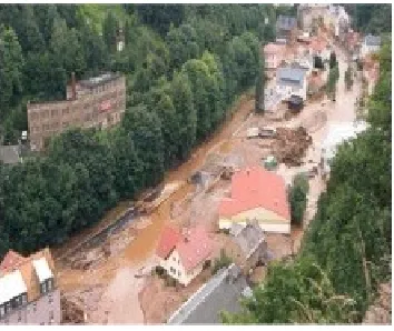
downstream reaches as shown in figure 1.2. Floods due to dam failure are
generally significantly larger than natural floods as unexpected high peak in
a different problem as compared to other natural floods Singh (2005). The
mitigation of the impacts of these possible risks, to the greatest possible degree
requires modelling of the flood with sufficient detail so as to capture both the
spatial and temporal evolution of the flood event. This therefore necessitates
the need of devising an appropriate model which can correctly simulate effects
of dam break failures, flood routing and sediment transport.
Figure 1.2: Flooding in Glashutte after the dam break in 12th August 2002
Source:http:espace.uq.edu.au/eserv/UQ:18350/chanson nova09.pdf.
1.3
Statement of the problem
Researchers have made significant contributions in the field of dam breaks
and bed load sediment transport but majority of them used Godunov type
methods in their simulations. Except Delis and Katsaounis (2005) who used the
relaxation schemes developed by Jin and Xin (1995) which is simple, requires
less computation time, achieves higher order accuracy and picks the right weak
solutions, see Jin and Xin (1995). However in their work they did simulations of
two mounds but in a confinement i.e the boundary conditions were all reflective
scenario as in our work, we simulate a situation that is more realistic. However
this study was motivated by the work of the researchers Delis and Katsaounis
(2005) and Simpson and Castelltort (2006) whereby the entrainment idea
of Simpson and Castelltort (2006) and the two mounds idea of Delis and
Katsaounis (2005) are combined to give more realistic simulations using the
relaxation schemes. A further step is taken, which is to simulate morphological
evolution of furrow located downstream of a breach location. Therefore in this
work we apply a finite volume discretization technique based on a relaxation
scheme to simulate the morphological evolution of the topography as a result
of a dam break, that causes flooding downstream of the breach location. The
considered mathematical model comprise of non-linear shallow water equations
coupled with bed-updating equations which take into account the entrainment.
The set of non-linear hyperbolic equations thus obtained are written in a
compact conservation form. The numerical modelling is done using the finite
volume, relaxation schemes. Using the relaxation approximation the non-linear
hyperbolic equations are converted to a linear hyperbolic system using the
relaxation variables V~ = (V1, V2, V3, V4), ~W = (W1, W2, W3, W4). The spatial
discretization is done using the Vanleer’s Monotone Upstream Centered Scheme
for Conservation Laws which is Time Variation Diminishing scheme,
(MUSCL-TVD). The time discretization (Full discretization) was done using the
implicit-explicit Runge-Kutta scheme. The capability of the model was tested by
performing simulations of two different scenarios namely;
1. The morphological evolution of a topographic surface with a deep narrow
2. The morphological evolution of a topographic surface with two mounds
located downstream of the breach location.
1.4
Hypothesis
1. The 2-D Shallow water equations (SWE) are adequate in describing the
considered flow problem.
2. The MUSCL-TVD method, a relaxation scheme despite being a
Riemann-solver free method, achieves a second order accuracy and picks up the
correct weak solutions in the solution of non-linear hyperbolic equations
(in two-phase flow problem) as compared to Riemann or
Godunov-type based methods which rely on approximate solutions of non-linear
Riemann problem and only yields first order accuracy.
1.5
Objectives
1.5.1
General objective
To simulate the morphological evolution of the topography as a result of a dam
break, that causes flooding downstream of the breach location.
1.5.2
Specific objectives
i.) To investigate effect of entrainment and bed-load transport on a
ii.) To investigate the effect of entrainment and bed-load transport on a
topographic surface with two mounds located downstream of the dam
break position.
1.6
Significance of the study
Dam break flows can cause serious flooding to downstream areas of the failed
structures. Flood waves resulting from dam breaks have been responsible for
severe losses of life and natural as well as man-made assets Hussain and Rai
(2000). As a result, the prediction of dam break flows is an essential part of
dam design, dam safety assessment, river flood control, water shed disaster
mitigation etc. The quality of dam break flow prediction mainly depends on
the appropriateness of mathematical formulation and the accuracy of numerical
simulation models.
The correct prediction of local sediment transport in the vicinity of structures
is an important research field due to its significant practical value as prediction
is necessary for calculation of the scouring risk of the structures and the
changes in the bed form. Several cases of the failure of structures exist where
correct prediction of local scour was not done Hudson and Sweby (2003).
Therefore accurate prediction of scour depth and its evolution in time is crucial.
Sediment transport is an area of major interest to various professionals, for
example the hydraulic engineers require this knowledge in the design of water
ways. The understanding of how sand interacts with the water flow in certain
environments such as coastal regions is also crucial to both the environment
and business. For example, if a harbour is constructed such that a considerable
and the costs of dredging the harbour may become too expensive and almost
impractical.
On the other hand sand can also be swept away from the beach resulting in only
coarse sand remaining. This can result in a massive decline in tourists visiting
the beach, and in turn severely affect the local community and businesses.
Therefore in this research we endeavor to develop a numerical model which can
possibly assist government agencies and other private institutions in conducting
flood risk assessment studies, planning and designing flood control projects and
establishing early warning systems and emergency actions.
1.7
Outline of the thesis
This thesis is organized into five chapters. Chapter two gives the literature
review of the related work done by other researchers in the field of simulation of
dam break flows and sediment transport on various channels. In chapter three
equations governing the flow are modelled, they comprise of the shallow water
equations and bed updating equations coupled with the entrainment. The
shallow water equations are derived from continuity equation and momentum
equations through the depth averaging and the long wave approximations.
These equations form a set of a non-linear hyperbolic partial differential
equations which are very difficult to solve analytically. Therefore a good choice
of the method of solving these system of equations has been carefully done. The
method chosen i.e. the relaxation method is robust, stable and accurately able
to capture the location of discontinuities such as shocks and contact surfaces
without using Riemann solvers. Unlike the relaxation scheme the Riemann
computer time. The relaxation method has simplicity and generality as its
main feature, it uses neither Riemann solver spatially nor non-linear systems of
algebraic equations solver temporally, yet it could achieve high order accuracy
and picks up the right weak solutions.
In Chapter four, the equations are formulated using the C formulation, an
unsteady approach which ensure that the Jacobian of the two flux matrices in
the x and y directions are non-singular. The resulting characteristic equation
is quite cumbersome and very difficult to solve because it contains several
variables and therefore we adopt the formula for the cubic function as given
by Spiegiel and Liu (1999). The relaxation is done by first converting the non
linear hyperbolic equations to linear hyperbolic equations using the relaxation
(artificial) valuables U, V, W. Spatial discretizations (semi-discretization) of
the linear hyperbolic equations was done using the Vanleer’s MUSCL-TVD
method, while the time discretization (full discretization) was done using the
fourth order implicit-explicit Runge-Kutta method.
Chapter five presents the results and the discussion of the research problem, it
is divided in four sections. Section one presents the initial and the boundary
conditions governing the research problem. In section two we present and
discuss the results for the effect of entrainment, morphological evolution and
bedload transport on the topographic surface having a narrow deep furrow. The
water depth contours, velocity vector plots, furrow profiles at three different
time intervals and the aerial view of the topographic surface before and after
morphological evolution have been presented. Section three provides the
transport on a topographic surface having two mounds downstream of the
breach location. In this section we have presented the water depth contours,
the vector velocity plots and the aerial view of the topographic surface before
and after morphological evolution the two mounds. While in section four the
conclusion of this study and the recommendations for future research works
are presented.
LITERATURE REVIEW
In this chapter we give an account of the related work which has been done
on simulation of dam break flows and sediment transport along the channels.
Zoppou and Stephen (1991) presented their work on catastrophic collapse
of water supply reservoirs in urban areas. In their study they developed a
model based on finite volume method combined with a first order approximate
Riemann solver to solve the two-dimensional shallow water wave equation
on an unstructured triangular grid. The model was applied to a case study
involving the sudden collapse of a water supply reservoir to predict the
progress of the flood ensuing from an instantaneous collapse of the reservoir.
The model was found to be conservative, robust, efficient, and capable of
simulating wetting and drying processes, resolving shocks, simulating flows
around complex geometries, and obstacles including influence of steep bed
slopes and friction.
Zhou et al. (2004) presented their work on numerical prediction of dam-break flows in general geometries with complex bed topography. In their work
they did numerical simulations of dam break flows in general geometries with
complex bed topography using a high-resolution Godunov-type cut cell method.
The model was based on shallow water equations with appropriate source
terms. A vertical step in the bed was treated efficiently and accurately with the
surface gradient method (SGM). For dam-break flows occurring in complicated
geometries, the Cartesian cut cell method together with transmissive boundary
conditions were incorporated. Verification of the model was carried out by
predicting dam-break flows typical of practical situations, i.e. dam break flows
over a vertical step into bent channels and a dam break flow over a bump in bed
with both transmissive and reflective boundary conditions at the channel end.
The results were compared with experimental data and showed good agreement.
Biscarini et al. (2010) presented their work on numerical simulations of free surface flows induced by a dam break comparing the shallow water approach
to fully three-dimensional simulations. The three-dimensional simulations were
based on the solution of the complete set of Reynolds-Averaged Navier-Stokes
(RANS) equations coupled to the volume of fluid (VOF) method. The methods
assessment and comparison were carried out on three scenarios namely a dam
break over a flat bed without friction, a dam break over a triangular bottom
sill and a dam break flow over a 900 bend. The results showed that the shallow water approach though was sufficiently able to reproduce the main aspects of
the fluid flows, loses some three- dimensional phenomena, due to the incorrect
shallow water idealization that neglects the three-dimensional aspects related
Singh et al. (2011) developed a two-dimensional numerical modelling of dam-break flows over natural terrain using a central explicit scheme. The governing
equations were modelled using the shallow water equations, the spatial
derivatives were discretized using a well-balanced explicit central upwind
conservative scheme while the time integration was performed using the Euler’s
scheme. The model was validated by simulating a laboratory experiment in
which a dam break flow propagates over a triangular obstacle and the model
was found to be satisfactory. A dam case laboratory experimental test case
on a friction-less horizontal bottom was also simulated for the 2-D validation
of the model, and a good agreement between simulation and experimental
data was observed. The suitability of the model for real life applications was
demonstrated by simulating the Malpasset dam-break event which occurred in
France in 1959. The computed arrival time of flood wave front and maximum
flow depths at various observation points matched well with the measurements
on a 4001 physical scale model.
The overall performance indicated that the model could be applied for
simulation of dam break flows in real life situation. Lachouette et al. (2009) presented their work on a numerical modelling of Interfacial soil erosion. In
their study they developed a numerical model for simulating the surface tension
occurring at a fluid/soil interface undergoing a flow process. The balance
equations with jump relations were used. A penalization procedure was used to
compute Stokes’s equations around obstacles, with a fictitious domain method,
in order to avoid body-fitted unstructured meshes and to use fast and efficient
evolution was described with a Level Set function. The ability of the model to
predict the interfacial erosion of soils was confirmed by presenting several 2-D
simulations.
Ahmadet al. (2013) presented their work on numerical method for dam break problem by using Godunov approach. They developed a numerical scheme
in order to overcome the problem of shock waves for the test case of a dam
break problem in one and two dimensions. The numerical scheme was based
on Godunov approach of finite volume method to solve the shallow water
equations. In order to expedite and improve the solution an approximate
Roe’s Riemann solver associated with monotone Upstream Centered Scheme
for Conservation Laws was applied. The results were presented in one and two
dimensions and verification were made with analytical solution. The results
were comparable and a good agreement was achieved between numerical and
analytical.
Audusse et al. (2013) presented their work on parallelization of a relaxation scheme, modeling the bed load transport of sediments in shallow water. They
did numerical simulations for bed load erosion processes. In their work they
presented a relaxation solver that could be applied to moving dunes test cases
in one and two dimensions which was not easy to handle at numerical level
especially when soft coupling (i.e. independent solvers or fluid and solid parts).
To run 2D test cases with reasonable CPU time they applied a parallelization
procedure by using domain decomposition based on the classical MPI library.
of irregular domains. In their work they developed a numerical technique for
the modelling of shallow water flow in one and two dimensions. The model
comprised of a cell-centered finite volume method based on Roe’s approximate
Riemann solver across the edges of both structured and unstructured cells.
The discretization of the bed slope source terms was done using an upwind
approach. The model was tested in different applications involving unsteady
flows in complex geometries such as dam break and advance over a triangular
obstacle, propagation of a smooth wave over a bump, non-symmetric dam break
in a pool with a pyramidal obstacle. The real life application was done by
simulating propagation of a flood wave in the Toce river physical model. These
results were validated with the successful comparison between the numerical
results and the experimental data.
Brufao and Navarro (2003) studied unsteady free surface simulation over
com-plex topography with a multidimensional upwind technique. They developed
a numerical model based on a first order upwind technique to solve one-and
two-dimensional problems for steady and unsteady free surface flows. The
model was tested in different applications involving unsteady flows in complex
geometries such as steady flow over a bump, dam break through a trapezoidal
breach, dam break in converging-diverging channel and steady flow in three
bumps. This numerical technique was validated with the successful comparison
between the numerical results and the experimental data.
Jean-Marie and Azzeddine (2010) presented a multi-dimensional upwind
topographies. They proposed a 2-D cell centered finite-volume scheme for
solving shallow water equations using both structured and unstructured fixed
meshes. Steady state C property and global mass conservation properties were
satisfied using appropriate numerical fluxes and wet/dry surface treatments.
The model was tested in different applications including idealized 1-D dam
break flow problems, Dam break on wet flat bottom, Dam break on dry flat
bottom and vacuum test with two expansion waves. The model was also applied
on a real case of wetting-drying simulations in a portion of the river ”Riviere
des prairies” in a suburb of Laval Quebec. With these validations the model
was found to be stable and robust.
Singh (2005) presented a two dimensional sediment transport model using
parallel computer that is, a vertically integrated two-dimensional numerical
sediment transport model. The sediment transport was simulated in two parts
namely, suspended load and bed load. He used the fractional step approach
to solve the two dimensional advection-diffusion equation which splits the
advection-diffusion equation in two separate parts i.e. advection and diffusion.
To solve advection part he used the high resolution conservative algorithm
and semi-implicit finite difference scheme to solve the diffusion part. To solve
the linear system of equations resulting from different diffusion part, parallel
numerical solvers were developed. He made the observation that the model
could simulate suspended load and bed load separately and that the bed load
transport is sensitive to different bed load transport capacity formulas and
capacity formula.
Brufaoet al. (2004) developed a 2D numerical model for dam break flows and achieved a zero mass error by modifying the wetting-drying condition which
included the normal velocity to the cell edges. Hudson and Sweby (2003)
investigated an accurate numerical solution of the equations governing
bed-load sediment transport. In their work they considered two approaches of
sediment flow namely the steady and unsteady approaches and compared the
accuracy of the formulations within their frameworks. They observed that
the formulation A−CV in the steady approach produced the most accurate
results though only to some limited values of the dimensional constant, Aand
the sediment transport flux q. Of the two approaches the unsteady approach
formulations were found to be more accurate than the steady approach and
on overall formulation C was found to be the most accurate as B could not
handle shocks in the cases of discontinuous flows. They observed that steady
approaches worked best when the Froude number, F r is small and when the
bed interacts slowly with the water flow while the unsteady approaches could
be used for all values of the dimensional constantAand the Froude numberF r.
Jin and Levermore (1996) studied numerical schemes for hyperbolic
conserva-tion laws with stiff source terms and showed through asymptotic analysis and
numerical examples that semi-discrete high resolution methods for hyperbolic
conservation laws fail to capture the asymptotic behavior unless the small
relaxation rate is reserved by a fine spatial grid. They introduced a modification
allowing the use of coarse grids (large cell peclets number).
Jin and Xin (1995) presented for the first time a new class of numerical
scheme known as the relaxation schemes for a system of conservation laws
in several space dimensions. They used a local relaxation approximation
to construct a linear hyperbolic system with a stiff lower order term that
approximates the original system with a small dissipative correction. Unlike the
then popular Godunov schemes such as upwind methods and central schemes
which relied on approximate solutions of non-linear Riemann problems, the
new linear hyperbolic system was solved by under-resolved stable numerical
discretizations, without using either Riemann solvers spatially or a non-linear
system of algebraic equation solvers temporally, yet it achieved high order
accuracy and picked the right weak solutions. The numerical results obtained
showed that the second order schemes are total variation diminishing (TVD)
in the zero relaxation limit for scalar equations.
Chalabi (1999) studied the convergence of relaxation schemes for hyperbolic
conservation laws with stiff source terms. He presented an analysis of a class
of relaxation schemes for hyperbolic conservation laws including stiff source
terms which had been introduced earlier, see Jin and Xin (1995) as explained
above in this literature. The construction of these schemes were based on the
approximation of an associated linear hyperbolic system with a stiff source term
depending on a small parametercalled relaxation time. This method avoided
the use of Riemann-solvers, and with an adequate and realistic hypothesis,
proposed semi-implicit and fully-implicit numerical schemes possessing good
properties such as monotony, TVD character, etc., exactly as in the case
of conservation laws without a source term q = 0 and showed that under
reasonable CFL conditions, the convergence of the approximate solution toward
a weak solution or to the entropy satisfying solution was established.
Delis and Katsaounis (2003) investigated a finite difference method for
calculating numerical solutions of the two dimensional shallow water systems
with source term based on bed topography. The method was based on
classical relaxation models combined with the TVD Runge-Kutta time stepping
mechanism where neither Riemann solvers nor characteristics decomposition
were used. The numerical results were presented for several test problems with
or without the the source term present. They observed that the method had
numerical dissipation especially while preserving steady states.
Delis and Katsaounis (2005)presented their work on the numerical solution
of two-dimensional shallow water equations by the application of relaxation
methods. They investigated a generalization and extension of a finite difference
method for calculating numerical solutions of the two dimensional shallow water
system of equations with source terms. The methods were based on classical
TVD Runge-Kutta time stepping mechanism where neither Riemann solvers
nor characteristics decomposition were needed. The presented numerical results
for several test problems with or without the source terms present such as
2-D partial dam break, circular dam break, steady flow over a hump, and a
showed that the relaxation schemes provide accurate solutions which were in
good agreement with well documented ones and besides having a comparable
resolutions with other well established methods they have simplicity as their
core advantage. This work was an improvement of his earlier work but this
time they devised novel ways of incorporating source terms with only small
errors being introduced while preserving steady states.
Diaz et al. (2008) presented their work on Sediment transport models in shallow water equations and numerical approach by high order finite volume
methods. In their work they focused on numerical approximation of bed load
transport due to water evolution and came up with a coupled model consisting
of hydrodynamic component and morphodynamic component. This model was
a set of non-conservative hyperbolic system of equations which were then solved
numerically using finite volume methods. These results were compared with
analytical solutions and experimental data and showed a good agreement.
Simpson and Castelltort (2006) presented a coupled model of surface water
flow, sediment transport and morphological evolution. The model was based
on shallow water equations for flow, conservation of sediment concentration,
and empirical functions for bed friction, substrate erosion and deposition.
The resulting hyperbolic system was solved using finite volume, Godunov-type
method with a first-order approximate Riemann solver. The developed model
could be used to investigate a variety of problems involving coupled flow and
sediment transport including channel initiation and drainage basin evolution
events such as tsunami.
From the cited literature review which has given an account of the contributions
in the field of dam breaks and sediment transport it is clear that majority
of researchers used Godunov type methods in their simulations, except Delis
and Katsaounis (2005) who used the relaxation schemes developed by Jin and
Xin (1995) which is simple, requires less computation time, achieves higher
order accuracy and picks the right weak solutions, see Jin and Xin (1995).
However in their work they did simulations of two mounds but in a confinement
i.e reflective boundaries and they never considered a breach. Therefore by
considering a dam break scenario as in our work, we simulate a situation that is
more realistic. However this study was motivated by the work of the researchers
Delis and Katsaounis (2005) and Simpson and Castelltort (2006) whereby the
entrainment idea of Simpson and Castelltort (2006) and the two mounds idea
of Delis and Katsaounis (2005) are combined to give more realistic simulations
using the relaxation schemes. A further step is taken, which is to simulate
THE GOVERNING
EQUATIONS
In this chapter we develop a mathematical model for a dam break and sediment
transport. This model is developed by coupling morphodynamic component
and hydrodynamic components. The hydrodynamic component is modeled by
shallow water equations while the morphodynamic component is modeled by
bed updating equation coupled with entrainment.
3.1
Derivation of Shallow Water equations
In this section we derive the shallow water equations with source terms due to
bed topography, frictional forces and entrainment. These equations are derived
from the principles of conservation of mass and conservation of momentum.
The independent variables are time t, and two space co-ordinates x and y,
while the dependent variables are the fluid height or depth h and the
2-dimensional fluid flow rates, hu and hv. With the proper choice of units,
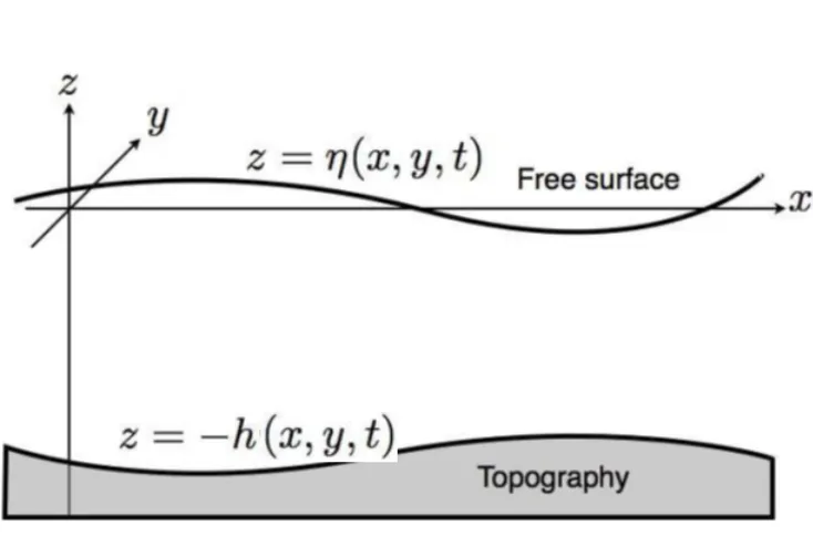
Figure 3.1: The Free surface Flow
the conserved quantities are mass, which is proportional to h, and momentum
which is proportional to u and v. The force acting on the fluid is gravity
represented by the gravitational constantg. The underlying assumption in the
derivation of these equations is that the depth of the fluid is small compared to
wave length of the disturbance. Since shallow water equations describe a thin
layer of fluid of constant density in hydrostatic balance, bounded from below
by bottom topography and above by a free surface the appropriate boundary
conditions will be stated and applied accordingly in the derivation of these
equations.
3.1.1
The conservation of Mass
This equation is based on two fundamental propositions:
i.) That the mass of the fluid is conserved i.e. it can neither be created nor
ii.) The flow is continuous and that empty spaces do not occur between
particles which were in contact
In differential form it is given as;
∂ρ
∂t +∇ ·(ρ~V) = 0 (3.1)
where ρ is the density andV~ = (u, v, w) is the velocity.
For an incompressible fluid (there is no variation of density with pressure).
Also, salinity and temperature can be assumed as constant. So fluid density,ρ
is constant in all the domain. Equation (3.1) becomes;
∇ ·V~ = 0 (3.2)
The equation (3.2) may be expressed as continuity equation. In differential
form in 3−D flow it takes the form;
∂u ∂x +
∂v ∂y +
∂w
∂z = 0 (3.3)
3.1.2
The Conservation of Momentum
Newton’s second law of motion is used to derive the equation of conservation
of momentum Andersonet al.(1984), in differential form the equation is given as;
∂(ρ~V)
∂t +∇ ·
h
ρ~V ⊗V~ +P I−Yi=ρg (3.4)
whereV~ is the velocity,ρis the density,P is the pressure,Q
is the viscosity
then Q
= 0 and the equation (3.4) becomes ;
∂(ρ~V)
∂t +∇ ·
h
ρ~V ⊗V~ +P Ii =ρg (3.5)
Since the fluid considered is incompressible then the equation (3.5) takes the
form;
∂ ~V
∂t +∇ ·
h
~
V ⊗V~i+1
ρ∇ ·P I =g (3.6)
Now adopting the convention that the horizontal plane is given by the
coordinates x and y and the vertical direction by z and also by denoting the
components of the body force vectors by g = (g1, g2, g3)=(0,0,-g) where g is
the acceleration due to gravity (assumed constant). Then the equation (3.6)
becomes
∂ ~V
∂t +∇ ·
h
~
V ⊗V~i+ 1
ρ∇ ·P I =
0 0 −g (3.7)
Rearranging equation (3.7), it takes the form
∂ ~V
∂t +∇ ·
h
~ V ⊗V~
i =−1
ρ∇ ·P I+
Equation (3.8) can be expressed in a more simplified form as;
∂u ∂t +u
∂u ∂x +v
∂u ∂y +w
∂u
∂z = −
1
ρ ∂p ∂x ∂v
∂t +u ∂v ∂x +v
∂v ∂y +w
∂v
∂z = −
1
ρ ∂p
∂y (3.9)
∂w ∂t +u
∂w ∂x +v
∂w ∂y +w
∂w
∂z = −
1
ρ ∂p ∂z −g
3.1.3
Boundary conditions
The mass continuity equation (3.3) and the conservation of momentum
equations (3.9) constitute the four equations with four unknowns i.e u, v, w
and p which by applying the appropriate boundary conditions may be solved
as spatial functions of x, y, z and time t.
The shallow water equations are approximations to free surface problem of
the figure 3.1. The boundary conditions for the free surface under gravity
Z =η(x, y, t) and the bottom surface Z =−B(x, y) are respectively;
D
Dt(η−Z) = 0 (3.10)
p=patm, (3.11)
wherepatm is the atmospheric pressure. At the bottom we have;
D
we also impose the no-slip condition at the bottom;
u=v = 0 (3.13)
Expanding the boundary conditions (3.10) we obtain;
(ηt+uηx+vηy −w)|z=η = 0 (3.14)
Expanding the boundary condition (3.12) in a similar way we get;
(uBx+vBy+w)|z=−B = 0 (3.15)
3.1.4
Boundary Layer Theory
The primary assumption in shallow water theory is that the horizontal scales
having wave lengthLare much larger than the vertical scales (in an undisturbed
water height).
We now analyse the equation of mass (3.3) as shown below;
∂u ∂x +
∂v ∂y
| {z } ≈u
l
+ ∂w
∂z
|{z} ≈w
h
= 0 (3.16)
and we deduce that
w≈uh
Where hl 1 and this leads to a boundary layer assumption;
∂w
∂t = 0 (3.18)
Now neglecting the vertical accelerations the system of equations (3.9) takes
the form;
∂u ∂t +u
∂u ∂x +v
∂u ∂y +w
∂u
∂z = −
1
ρ ∂p ∂x ∂v
∂t +u ∂v ∂x +v
∂v ∂y +w
∂v
∂z = −
1
ρ ∂p
∂y (3.19)
∂w
∂t = −
1
ρ ∂p ∂z −g
and now applying the boundary layer assumption equation (3.18) unto equation
(3.19) we get;
∂u ∂t +u
∂u ∂x +v
∂u ∂y +w
∂u
∂z = −
1
ρ ∂p ∂x ∂v
∂t +u ∂v ∂x +v
∂v ∂y +w
∂v
∂z = −
1
ρ ∂p
∂y (3.20)
0 = −1
ρ ∂p ∂z −g
3.1.5
Hydrostatic Pressure
The vertical component of equation (3.20) can be re-written as;
∂p
integrating equation (3.21) with respect to z we get the following hydostatic
pressure relation;
p=g
Z η z
ρdz+pa (3.22)
Assuming constant density along the z axis the equation (3.22) becomes;
p=ρg(η−z) +pa (3.23)
Differentiating equation (3.23) with respect to x we get the pressure gradient
along the xdirection as;
∂p ∂x =ρg
∂η
∂x (3.24)
Similarly, differentiating the same equation (3.23) with respect toy we get the
pressure gradient along the y direction as;
∂p ∂y =ρg
∂η
∂y (3.25)
and hence from the equations (3.24) and (3.25), it’s clear that the hydrostatic
pressure relation (3.22) is independent of the variablez and therefore it is only
responsible for the horizontal accelerations;
3.1.6
Horizontal Mean Velocity
The horizontal velocitiesuand v are independent of the variablez and can be
interpreted as the vertical mean velocities and therefore can be written in the
form;
∂u ∂z =
∂v
3.1.7
The simplified Momentum Equations
Putting equation (3.24) and (3.26) in the first of the equations (3.20), equation
(3.25) and (3.26) in the second of the equation (3.20) we get the following set
of equations;
∂u ∂t +u
∂u ∂x +v
∂u ∂y =−g
∂η
∂x (3.27)
∂v ∂t +u
∂v ∂x +v
∂v ∂y =−g
∂η
∂y (3.28)
3.1.8
Depth Averaging
Now integrating the continuity equation vertically;
Z η −B
∇ ·V dz~ = 0,−B < Z < η (3.29)
Expanding the continuity equation, we get;
0 = Z η −B ∂u ∂x + ∂v ∂y + ∂w ∂z dz (3.30)
. We now apply the Leibintz rule of integration to integrate equation (3.30),
we obtain;
0 = ∂
∂x
Z η −B
udz−u|z=η
∂η
∂x +u|z=−B
∂(−B)
∂x
+ ∂
∂y
Z η −B
vdz−v|z=η
∂η
∂y +v|z=−B
∂(−B)
∂y (3.31)
And now putting (3.15) into (3.31) the above equation becomes;
0 = ∂
∂x
Z η −B
udz−u|z=η
∂η ∂x
+ ∂
∂y
Z η −B
vdz−v|z=η
∂η
∂y (3.32)
+ w|z=η
Now applying the boundary conditions (3.14) to the equation (3.32) we get;
∂η ∂t +
∂ ∂x
Z η −B
udz+ ∂
∂y
Z η −B
vdz = 0 (3.33)
. Sinceu and v are independent of z then the equation (3.33) becomes;
∂η ∂t +
∂[(η+B)u]
∂x +
∂[(η+B)v]
∂y = 0 (3.34)
. Assuming that in this particular case that B(x, y) is independent of time
then it implies that Bt= 0 and therefore we can write the equation (3.34) as;
(η+B)t+ [u(η+B]x+ [v(η+B)]y = 0 (3.35)
Now multiplying the equation (3.35) by u and adding to equation (3.27)
pre-multiplied by (η+B), we obtain;
Similarly multiplying equation (3.35) byv and then add to the equation (3.28)
pre-multiplied by (η+B) we obtain;
[v(η+B)]t+ [uv(η+B]x+ [v2(η+B)]y =−g(η+B)ηy (3.37)
The right hand side of equation (3.36) can be expanded as follows;
−g(η+B)ηx=g(η+B)Bx− 1
2g[(η+B)
2]
x (3.38)
Expanding the right hand side of equation (3.37) we obtain;
−g(η+B)ηy =g(η+B)By− 1
2g[(η+B)
2]
y (3.39)
Putting (η+B) = hwhere his the total water height then the equation (3.35)
takes the form;
ht+ (hu)x+ (hv)y = 0 (3.40)
Again letting (η+B) = h and expanding the right hand side of the equation
according to (3.36) we obtain;
(hu)t+ (hu2+ 1 2gh
2)
x+ (huv)y =−ghBx (3.41)
Similarly expanding the right hand side of the equation (3.37) while letting
(η+B) =h we obtain;
(hv)t+ (huv)x+ (hv2+ 1 2gh
2)
3.1.9
The Final form of Shallow Water Conservation
Equations (Hydrodynamics Equations)
The equation of continuity (3.40) and the equations of the conservation of
momentum (3.41) and (3.42) combined together form a set of system of
equations in conservation form;
ht+ (hu)x+ (hv)y = 0 (hu)t+ (hu2+
1 2gh
2)
x+ (huv)y = −ghBx (3.43) (hv)t+ (huv)x+ (hv2 +
1 2gh
2)
y = −ghBy
wherehis the height of the water,uand v are the depth averaged velocities in
the x and y directions respectively and B =B(x, y) is the function describing
the bottom profile. We can now express the system of shallow water equations
(3.43) in a more compact conservation form as follows;
Ut0 +F0(U0)x+G0(U0)y =S0(U0) (3.44)
where;
U0 = [h, hu, hv]T is the vector of the conserved variables,
F0(U0) = [hu2, hu2+12gh2, huv]T is the flux in the x direction
G0(U0) = [hv, huv, hv2+ 12gh2]T is the flux in the y direction and
3.1.10
Bed-updating Equation
When deriving this equation, we assume that height of the river bed denoted
by B , is not stationary. We therefore express it as function of the space
coordinates x, y and time t i.e
B =B(x, y, t) (3.45)
and take the boundary condition as;
D
Dt(Z−B) = 0 (3.46)
. Now using the definition of the material derivative we can expand the
boundary condition (3.46) as follows;
Bt+uBx+vBy −w|z=B = 0 (3.47)
. Integrating the bed-update equation vertically we get;
Z B
0
∇ ·V dz~ = 0 (3.48)
. Expanding the equation (3.48), we write it as;
Z B
0
∂u ∂x +
∂v ∂y +
∂w ∂z
. Integrating equation (3.49) using the Leibntz rule we get;
0 = ∂
∂x
Z B
0
udz−u|z=B
∂B ∂x
+ ∂
∂y
Z B
0
vdz−v|z=B
∂B
∂y +vz=B ∂(B)
∂y (3.50)
+ w|z=B−w|z=0
Substituting the expanded boundary condition (3.47) to equation (3.50), we
get;
Bt+
∂ ∂x
Z B
0
udz+ ∂
∂y
Z B
0
vdz = 0 (3.51)
Equation (3.51) may be expressed in the form;
Bt+
∂
∂x(Bu)dz+ ∂
∂y(Bv)dz = 0 (3.52)
The volumetric load transport in x and y directions according to (Kaushik
2005) is respectively expressed as;
Bu=ξp1 (3.53)
Bv =ξp2 (3.54)
Where;
ξ= 1−1 and is the porosity of the furrow
Now putting (3.53) and (3.54) into equation (3.52), we get the bed updating
equation;
∂ ∂tB+ξ
∂
∂x(p1) +ξ ∂
In our case we are interested with the bed load sediment transport and its
effects such as entrainment on various topographies. Various scientist have
come up with numerous analytical sediment transport formula of which the
choice depends on the particular situation being modeled. In our work we shall
adopt the one derived by Grass (1981) because it is a simple model and the
critical shear stress is set to zero;
p1 =Au(u2+v2)
m−1
2 (3.56)
p2 =Av(u2 +v2)
m−1
2 (3.57)
Where A is a dimensional constant sm2,( where s is the specific gravity) which encompasses the effects of the grain size and kinematic viscosity which is being
chosen from an experimental data. We observe that the equations (3.56) and
(3.57) can only be differentiated with respect to u and v respectively only if
they are not allowed to change signs.
However, by considering the odd integers of m only then the equations (3.56)
and (3.57) can be differentiated and become valid for all values of u and v
and hence for this reason we shall use the value of m = 3 as it is the smallest
3.1.11
The Final form of the Governing Equations
(Morphodynamic Equations)
In this research we shall adopt the following formula for entrainment as given
by Simpson and Castelltort (2006);
E0 =β
" p
(u2+v2)
uc
−1 #γ
(3.58)
Where β is the entrainment coefficient, uc is a threshold entrainment flow velocity (Izumi and Parker 2000)and therefore the continuity equation becomes;
ht+ (hu)x+ (hv)y =
E0
1−φ (3.59)
. Similarly the updating equation becomes;
∂ ∂tB+ξ
∂ ∂p1+ξ
∂ ∂p2 =
E0
1−φ (3.60)
whereξis the bed sediment porosity. Now considering the effects of the friction
on thex and y directions and incorporating in momentum equations, we get;
(hu)t+ (hu2+ 1 2gh
2
)x+ (huv)y =−ghBx−ghSf x (3.61)
(hv)t+ (huv)x+ (hv2+ 1 2gh
2
)y =−ghBy −ghSf y (3.62)
Now coupling the derived shallow water equations to the equations for the
sediment transport.
ht+ (hu)x+ (hv)y =
E0
1−φ
(hu)t+
hu2+ 1 2gh
2
x
+ (huv)y = −ghBx−ghSf x (3.63)
(hv)t+ (huv)x+
hv2+1 2gh
2
y
= −ghBy−ghSf y
∂ ∂tB +ξ
∂
∂x(p1) +ξ ∂
∂y(p2) = E0
1−φ
where the friction forces in the two respective direction is as given by the
Darcy-Weisbach equation;
Sf x=
f u√u2+v2
8gh , Sf y=
f v√u2 +v2
8gh (3.64)
wheret is the time, xand y are horizontal coordinates, his the flow depth , u
and v are depth-averaged velocities in the x and y directions respectively Bx and By are the bed topographic elevations while p1 and p2 are the volumetric
sediment transport rates in thexand y respectively. The equations (3.63) and
(3.64) form the complete system of equations governing the sediment transport
in two dimensions.
3.1.12
Non-dimensionalization
The non-dimensionalization process is important because the results obtained
for a surface experiencing one set of conditions can be applied to a geometrically
similar surface experiencing entirely different conditions. Conditions may vary
with the nature of fluid, the fluid velocity or the size of the surface. The process
In this study the non-dimensionalization will be based on the following sets of
scaling variables.x =x∗L, y = y∗L, t =t∗T, h= h∗L, B = B∗L, g = TL2g
∗, v =
L Tv
∗, u= L Tu
∗ whereL=max
i,j(|xi,j−x0,j, yi,j−yi,0|) and T =
q L g
Writing the first equation of (3.63) in in non-dimensional form, we get;
L T
∂h∗ ∂t∗ +
L T
∂h∗u∗
∂x∗ +
L T
∂h∗v∗ ∂y∗ =
E0
1−φ ∂h∗
∂t∗ +
∂h∗u∗
∂x∗ +
∂h∗v∗ ∂y∗ =
T L
E0
1−φ ∂h∗
∂t∗ +
∂h∗u∗
∂x∗ +
∂h∗v∗ ∂y∗ =
1 √
gL E0
1−φ
(3.65)
Writing the second equation of (3.63) in a non-dimensional form, we get;
L2 T2
∂h∗u∗ ∂t∗ +
1 L ∂ ∂x∗ L3 T2h
∗
u∗2+ L
3
2T2g
∗
h∗2
+ 1 L ∂ ∂y∗ L3 T2h
∗
u∗v∗
= −L
3
LT2
∂B∗ ∂x∗ −
L2
T2g
∗
h∗sf x
L2 T2
∂h∗u∗ ∂t∗ +
L2 T2
∂ ∂x∗
h∗u∗2+1 2g
∗
h∗2
+ L
2
T2
∂ ∂y∗ (h
∗
u∗v∗)
= L
2
T2
∂B∗ ∂x∗ −g
∗
h∗sf x
∂h∗u∗ ∂t∗ +
∂ ∂x∗
h∗u∗2+1 2g
∗
h∗2
+ ∂
∂y∗ (h ∗
u∗v∗)
=
∂B∗ ∂x∗ −g
∗
h∗sf x
Writing the third equation of (3.63) in non-dimensional form, we get;
L2 T2
∂h∗v∗ ∂t∗ +
1 L ∂ ∂x∗ L3 T2h
∗
u∗v∗
+ 1 L ∂ ∂y∗ L3 T2h
∗
v∗2+ L
3
2T2g
∗
h∗2
= −L
3
LT2
∂B∗ ∂y∗ −
L2
T2g
∗
h∗sf y
L2
T2
∂h∗v∗ ∂t∗ +
L2
T2
∂ ∂x∗ (h
∗
u∗v∗) + L
2
T2
∂ ∂y∗
h∗v∗2+ 1 2g
∗
h∗2
= L 2 T2 ∂B∗ ∂y∗ −g
∗
h∗sf y
∂h∗v∗ ∂t∗ +
∂ ∂x∗ (h
∗
u∗v∗) + ∂
∂y∗
h∗v∗2+1 2g
∗
h∗2
=
∂B∗ ∂y∗ −g
∗
h∗sf y
(3.67)
and finally writing the fourth equation of (3.63) in a non-dimensional form we
have;
L T
∂B∗
∂t∗ + ξ
T2 L 1 L L3 T3
∂p∗1 ∂x∗ +ξ
T2 L 1 L L3 T3
∂p∗2 ∂x∗ =
E0
1−φ ∂B∗
∂t∗ + ξ
∂p∗1 ∂x∗ +ξ
∂p∗2 ∂y∗ =
T L
E0
1−φ ∂B∗
∂t∗ + ξ
∂p∗1 ∂x∗ +ξ
∂p∗2 ∂y∗ =
1 √
gL E0
1−φ
Now dropping the superscripts the set of the specific governing equations in
the non-dimensional form are;
ht+ (hu)x+ (hv)y =
E
1−φ
(hu)t+
hu2+1 2gh
2
x
+ (huv)y = −ghBx−ghsf x (3.69)
(hv)t+ (huv)x+
hv2+ 1 2gh
2
y
= −ghBy −ghsf y
∂ ∂tB+ξ
∂
∂x(p1) +ξ ∂
∂y(p2) = E
1−φ
where,E =β0
√ u2+v2
uc −1
γ
NUMERICAL METHODS
In this chapter we write the set of the non-linear hyperbolic conservations laws
derived in the previous chapter, using the C formulation. The advantage of
writing the conservation laws using this formulation is that it ensures that
the Jacobian of the flux matrices F(U) and G(U) i.e. ∂F∂U(U) and ∂G∂U(U) are non-singular and therefore their respective eigenvalues and their corresponding
eigen vectors could be determined. To solve the characteristics equations
associated with the Jacobian matrices we use the cubic polynomial formula
as given by Spiegiel and Liu (1999). The eigenvalues determined were found
to be real and unequal and this demonstrates that the set of system of the
nonlinear partial differential equations derived are hyperbolic in nature. These
systems of equations admits steady-state solutions in which the non-zero flux
terms are balanced by the source terms and also admit solutions that involve
discontinuous and non-linear waves, such as shocks and rarefactions as well as
wet-dry interfaces generated by dam break flows.
This set of hyperbolic partial differential equations are quite difficult to solve
analytically and therefore have to be solved using a suitable numerical method,
one which produces low numerical dissipation and diffusion. There are several
numerical schemes which can be used to solve these equations such as upwind
methods which rely on approximate solutions of non-linear Riemann problems,
central schemes also known as Godunov-type schemes on staggered grids, etc.
In this work we shall use a more stable, accurate, simple to use, having
comparatively less computer time usage and quite robust schemes called
the relaxation schemes. This scheme is based on an approximation on the
continuous level before performing the discretizations leading to high-resolution
and Riemann solver free methods. The method is also important because it
can handle complicated system of conservation laws such as two-phase flow
problems like the one in consideration, where we don’t expect to have an
analytical expression for the physical flux. The main idea behind the relaxation
method is to use a local relaxation approximation, by constructing a linear
hyperbolic system with a stiff lower order term that approximates the original
nonlinear system with a small dissipative correction. The new system can
then be solved by under-resolved stable numerical discretizations without using
either Riemann solvers spatially or a non-linear system of algebraic equations
solver temporally.
Once we have modeled the equations using the C formulation and obtained
the eigenvalues, the non-linear hyperbolic equations are converted to a linear
equilibriums in the relaxation limits → 0+. Introducing the relaxation
variables U, V, W a relaxation model is developed to relax the non linear
hyperbolic equations. Once the equations have been relaxed we then perform
semi-discretization i.e spatial discretization using the Vanleers MUSCL scheme.
This scheme is quite powerful and it yields second order accurate in space
scheme unlike the upwind stream schemes, see Jin and Xin (1995). Finally
we complete the discretization by performing time discretization. To ensure a
high order accurate results in time discretization we shall use the fourth order
implicit-explicit Runge-Kutta splitting schemes. The splitting treats the source
terms implicitly in two steps i.e due to linearity ofV and W and then solved
explicitly, and the convective terms with two explicit steps. Thus, we have
an explicit implementation of implicit source terms, solely determined by the
non-stiff convection terms, just as in a usual shock capturing scheme.
At the end of this chapter we specify the initial and the boundary conditions
for the dam break scenario having a topography with a narrow deep furrow
on downstream location of the breach and a a dam break scenario having
topography with two mounds on the downstream location of the breach
location.
4.1
C-Formulation
There exists two approaches of rewriting the governing equations in