On the estimation of intracluster correlation for time-to-event outcomes in cluster randomized trials

(1)

Western University Western University

Scholarship@Western

Electronic Thesis and Dissertation Repository

8-28-2015 12:00 AM

On the estimation of intracluster correlation for time-to-event

outcomes in cluster randomized trials

Sumeet Kalia

The University of Western Ontario

Supervisor Dr. Allan Donner

The University of Western Ontario Joint Supervisor Dr. Neil Klar

The University of Western Ontario

Graduate Program in Epidemiology and Biostatistics

A thesis submitted in partial fulfillment of the requirements for the degree in Master of Science © Sumeet Kalia 2015

Follow this and additional works at: https://ir.lib.uwo.ca/etd

Part of the Biostatistics Commons

Recommended Citation Recommended Citation

Kalia, Sumeet, "On the estimation of intracluster correlation for time-to-event outcomes in cluster randomized trials" (2015). Electronic Thesis and Dissertation Repository. 3213.

https://ir.lib.uwo.ca/etd/3213

This Dissertation/Thesis is brought to you for free and open access by Scholarship@Western. It has been accepted for inclusion in Electronic Thesis and Dissertation Repository by an authorized administrator of

(2)

ON THE ESTIMATION OF INTRACLUSTER CORRELATION FOR

TIME-TO-EVENT OUTCOMES IN CLUSTER RANDOMIZED TRIALS

(Thesis format: Monograph)

by

Sumeet Kalia

Graduate Program in Department of Epidemiology and Biostatistics

A thesis submitted in partial fulfillment

of the requirements for the degree of

Masters of Science

The School of Graduate and Postdoctoral Studies

The University of Western Ontario

London, Ontario, Canada

c

(3)

Abstract

Cluster randomized trials (CRTs) involve the random assignment of intact social units

rather than independent subjects to intervention groups. Time-to-event outcomes often are

endpoints in CRTs where the intracluster correlation coefficient (ICC) serves as a descriptive

parameter to assess the similarity among outcomes in a cluster. However, estimating the ICC in

CRTs with time-to-event outcomes is a challenge due to the presence of censored observations.

The ICC is estimated for two CRTs using the censoring indicators and observed outcomes.

A simulation study explores the effect of administrative censoring on estimating the ICC.

Results show that the ICC estimators derived from censoring indicators and observed outcomes

are negatively biased for positively correlated outcomes. Analytic work further supports these

results. Censoring indicators may be preferred to estimate the ICC under moderate frequency

of administrative censoring while the observed outcomes may be preferred under minimal

fre-quency of administrative censoring.

Keywords: Cluster randomized trials; intracluster correlation coefficient; correlated

time-to-event outcomes; multivariate exponential distribution.

(4)

Acknowledgments

I am indebted to my supervisors, Dr. Allan Donner and Dr. Neil Klar. This thesis would

not be possible without their guidance and support.

I am sincerely grateful to Dr. Guangyong Zou, Dr. Greta Bauer, Dr. Igor Karp and other

faculty members for the invaluable lectures in Epidemiology and Biostatistics.

I would like to thank my friends and student colleagues for providing an intellectually

stimulating environment. I would also like to thank my family for the support they provided

me through my entire life.

This work was financially supported, in part, by an Ontario Graduate Scholarship and Dr.

Donner’s Natural Sciences and Engineering Research Council grant.

(5)

List of Figures

5.1 Mean ICC estimate for case 1:ρ=0,m=200,k=40 . . . 35

5.2 Variance of ICC estimators for case 1:ρ=0,m=200,k=40 . . . 36

5.3 Mean square error of ICC estimators for case 1:ρ=0,m=200,k=40 . . . . 37

5.4 Mean between-cluster variance component for case 1:ρ=0,m=2,k=40 . . 38

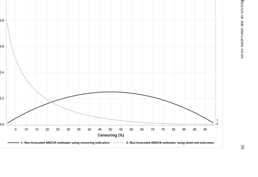
5.5 Mean within-cluster variance component for case 1:ρ=0,m=200,k=40 . . 39

5.6 Sign test for case 1: ρ=0,m=2,k=40 . . . 40

5.7 Mean ICC estimate for case 2:ρ=0.01,m=200,k=40 . . . 41

5.8 Variance of ICC estimators for case 2:ρ=0.01,m=200,k=40 . . . 42

5.9 Mean square error of ICC estimators for case 2:ρ=0.01,m=200,k=40 . . . 43

5.10 Mean between-cluster variance component for case 2: ρ=0.01,m=200,k=40 44 5.11 Mean within-cluster variance component for case 2: ρ=0.01,m=200,k=40 45 5.12 Sign test for case 2: ρ=0.01,m=200,k=40 . . . 46

5.13 Mean ICC estimate for case 3: ρ=0,m=2,k=40 . . . 48

5.14 Variance of ICC estimators for case 3: ρ=0,m=2,k=40 . . . 49

5.15 Mean square error of ICC estimators for case 3: ρ=0,m=2,k=40 . . . 50

5.16 Mean between-cluster variance component for case 3: ρ=0,m=2,k=40 . . 51

5.17 Mean within-cluster variance component for case 3: ρ=0,m=2,k=40 . . . 52

5.18 Sign test for case 3: ρ=0,m=2,k=40 . . . 53

5.19 Mean ICC estimate for case 4: ρ=0.01,m=2,k=40 . . . 54

5.20 Variance of ICC estimators for case 4: ρ=0.01,m=2,k=40 . . . 55

5.21 Mean square error of ICC estimators for case 4: ρ=0.01,m=2,k=40 . . . . 56

5.22 Mean between-cluster variance component for case 4: ρ=0.01,m=2,k=40 . 57 5.23 Mean within-cluster variance component for case 4: ρ=0.01,m=2,k=40 . . 58

5.24 Sign test for case 4: ρ=0.01,m=2,k=40 . . . 59

5.25 The mean of non-truncated ICC estimator (solid gray line) and ICC parameter (solid black line) derived from censoring indicators . . . 61

5.26 The correlation between non-truncated ICC estimators using censoring indica-tors and observed outcomes . . . 62

6.1 Cumulative-incidence of childhood mortality in bednet and control group. . . . 66

6.2 Cumulative-incidence of tube failure in prednisone and sulfamethoprim, and placebo group. . . 68

(9)

List of Tables

2.1 Literature review for the use of ICC . . . 16

3.1 The joint and marginal probabilities of censoring indicators . . . 21

4.1 Parameter combinations of the simulation study . . . 26

4.2 The ANOVA ICC estimators of the simulation study . . . 28

5.1 Mean bias of ANOVA ICC estimator in the absence of censoring . . . 33

5.2 The summary of mean bias whenm=200 . . . 34

5.3 The summary of mean bias whenm=2 . . . 47

5.4 Summary of disparity (=_bρc−ρc) for the four cases. . . 60

5.5 Summary of Corr(_bρc,bρt) . . . 60

6.1 Summary statistics for the control and bednet group. . . 66

6.2 The ANOVA ICC estimates of control and bednet group. . . 67

6.3 Summary statistics for prednisone and sulfamethoprim, and placebo group . . . 68

6.4 The ANOVA ICC estimates of Placebo and prednisone and sulfamethoprim group. . . 69

A.1 One-way random effects model . . . 82

(10)

List of Acronyms

ANOVA analysis of variance

CRTs cluster randomization trials

ICC intracluster correlation coefficent

ML maximum likelihood

MSB between mean sums of squares

MSE mean square error

MSW within mean sums of squares

REML restricted maximum likelihood

SSB between sum of squares

SST total sum of squares

SSW within sum of squares

VIF variance inflation factor

(11)

Chapter 1 Introduction

Randomized trials are prospective studies designed to evaluate the effectiveness of a given

intervention (Friedman et al., 2010). The random assignment of individual subjects ensures

that, on average, the intervention groups are comparable with respect to both known and

un-known baseline risk factors. In addition, random assignment helps to prevent selection bias

that may originate from participants or investigators who may have a preference for one of the

interventions being evaluated.

1.1 Cluster randomized trials

Investigators may at times choose to randomize intact social units (or clusters) instead of

individual subjects (Donner and Klar, 2000, p. 5). Some possible benefits of randomizing

clusters include reduced treatment contamination, increased administrative convenience, and

improved participant compliance. In one example, investigators chose to randomize Hutterite

colonies to evaluate the effect of influenza vaccine on infection rates (Loeb et al., 2010). The

adoption of this design assured that possible treatment contamination of influenza vaccine

ef-fects under individual randomization is minimized in each colony.

The development of cluster randomization trials (CRTs) has independently arisen in

(12)

Chapter1. Introduction 2

ious disciplines including medicine, social science, psychology and educational research. In

the medical literature, there was an early recognition of decreased precision associated with

CRTs, e.g. Mainland (1952, p. 114). Despite this early acknowledgment, many researchers

continue to face difficulties with the design and analysis of CRTs. This is demonstrated in

sev-eral methodological reviews including Simpson et al. (1995), Smith et al. (1997), and Walleser

et al. (2011). In many instances, investigators may not be aware of the need to account for

clustering and thus inappropriately choose standard statistical procedures to evaluate the

inter-vention effect. However, it has been shown numerous times that the results derived from na¨ıve

methods ignoring clustering can often be misleading (Donner and Klar, 2000, p. 85, 113, 129).

This is because the fundamental assumption of independence among outcomes no longer holds

and therefore the use of standard statistical procedures is invalid. In particular, the estimated

variance obtained from standard statistical procedures assuming all outcomes are independent

underestimates the true variance and this leads to exaggerated effects of statistical significance.

The design of CRTs can also be severely hampered if the sample size is estimated through

standard statistical procedures because this may give rise to an inconclusive study with low

power.

The most common experimental designs used in CRTs include the completely randomized,

pair-matched and stratified designs. The completely randomized design randomly assigns

clus-ters to the intervention groups without any matching or stratification. This design is most

suit-able when a large number of clusters are availsuit-able since in this case effective randomization

can ensure that both known and unknown baseline risk factors are, on average, balanced across

the intervention groups. An example of a completely randomized design comes from a study

of neonatal intensive care units where 114 hospitals were randomized to the intervention or

control group (Horbar et al., 2004). The pair-matched design involves matching clusters on the

(13)

one cluster at random to the intervention group and the other cluster to the control group. As

an example, 14 nursing homes were pair-matched on the basis of total number of beds and

geo-graphical proximity to evaluate an intervention program designed to prevent injuries among the

residents (Ray et al., 1997). The stratified design is simply an extension of the pair-matched

design where several clusters within each stratum are randomly assigned to the intervention

group or control group. For example, each Hutterite colony within the seven health regions

classified as a strata were randomized to one of the two treatment groups (Loeb et al., 2010).

The rationale for adopting the pair-matched and stratified designs is that the probability of

im-balance on important baseline characteristics can be substantially greater in trials randomizing

clusters than for individually randomized trials with the same number of participants (Donner,

1992). Although an extensive literature exists on each of these designs, the focus here will be

limited to the completely randomized design.

Many CRTs involve the collection of correlated data consisting of the time to a specified

event. For example, Loeb et al. (2010) examined the time to laboratory confirmed influenza

cases among the members of Hutterite communities. Outcomes were considered to be

ad-ministratively censored if a given individual did not acquire influenza during the follow up of

the trial. In addition, censored observations could arise if clusters or individual participants

were lost to follow-up, chose to dropout or acquired a competing event which precluded

ob-serving the primary endpoint. For the sake of simplicity, the focus in this thesis is limited to

administrative censoring where the assumption of non-informative censoring is satisfied.

Non-informative censoring can be defined as independence between event times and the censoring

mechanism possibly conditioned on a set of covariates (Wax et al., 1993). As a consequence,

this assumption ensures that the probability of being censored does not depend on the prognosis

of a subject or a cluster (Kleinbaum and Klein, 2012).

(14)

types of accrual schemes in CRTs: (1) recruiting clusters sequentially while recruiting subjects

simultaneously, (2) recruiting clusters simultaneously while recruiting subjects sequentially

and (3) recruiting both clusters and subjects sequentially in relation to randomization. In an

ideal design of CRT, the identification and recruitment of participants must be done prior to

the random assignment (Eldridge et al., 2009). This design feature reduces the possibility

of selection bias which may arise from differential rates of recruitment across intervention

groups. Hence the focus in this thesis is limited to the accrual scheme where both the clusters

and subjects are assumed to be available at the start of the trial. This focus in combination with

limiting attention to administrative censoring simplifies the design and analysis of simulation

study described in chapters 4 and 5. As an example, subjects within each Hutterite communities

were recruited prior to the randomization of the study (Loeb et al., 2010). In addition, trial

researchers (e.g. recruiters, assessors etc.) and subjects should also be blinded (whenever

ethically possible) to the allocation status to reduce other sources of systematic error.

1.2 Intracluster correlation coe

ffi

cient

The lack of independence among outcomes observed on cluster members creates statistical

challenges that may be accounted for using an estimator of the parameter ρ, where ρ

mea-sures the degree of similarity among outcomes within a cluster and is known as the intracluster

correlation coefficent (ICC). The ICC has a rich history of application in various fields of

research (Haggard, 1958). For example, it may be used to measure familial resemblance in

epidemiological studies, heritability of traits in genetic studies, and reliability of assessors in

psychological studies (Donner, 1986). The ICC was first defined as a descriptive measure “to

determine the resemblance for any series of characters of the individuals of sub-classes. . . as

compared to the random pairs from the population (or universe) which they constitute”

(Har-ris, 1913). Although the estimation of ICC’s was first established for continuous endpoints

(15)

(Ridout et al., 1999) and time-to-event (Xie and Waksman, 2003).

1.2.1 Continuous outcomes

Pearson product-moment correlation can be used to estimate the ICC for continuous

out-comes and it is defined in the present context as the pairwise correlation between any two

members of the same cluster where each distinct pair of members is counted twice. However,

as noted by Donner (1986), the pairwise correlation loses efficiency when substantial variation

exists in the size of the clusters. For example, consider the Loeb et al. (2010) trial where the

total number of subjects per cluster varied from 11 to 123. In this case, the group consisting

of 123 subjects would be weighted approximately 136 times more than the group consisting

of 11 subjects

i.e.(

123 2 )

(11 2)

136

. The magnitude of this weight is the ratio of two permutations

that enumerate the total number of pairs. In order to overcome this disadvantage, a weighted

pairwise correlation can be constructed as proposed by Karlin et al. (1981). The weights may

be constructed so that (i) each pair of observations has equal weight, (ii) each group has equal

weight regardless of their sizes, or (iii) each pair is weighted depending on the total number of

pairs in which the given individual appears.

Fisher (1925) recognized that the ICC “merely measures the relative importance of two

groups of factors causing variation” and hence introduced analysis of variance (ANOVA) to

estimate the ICC based on what now is denoted a one-way random effects model. The ANOVA

partitions the overall variance into two factors: (1) within-cluster and (2) between-cluster

variance and directly estimates the ICC as the proportion of total variation accounted for by

between-cluster variation. In the case of fixed cluster size (i.e. same number of subjects per

cluster), the ANOVA estimator of variance components has many appealing properties. For

example, the ANOVA estimators of variance components are unbiased and under normality

have the minimum variance among all unbiased estimators (Searle et al., 1992, p. 129, 175

(16)

of variance components does not equal to the ratio of expected variance components (Ponzoni

and James, 1978). Furthermore, in the case of variable cluster size where the between-cluster

variance component is greater than the within-cluster variance component or equivalentlyρis

greater than half, the performance of the ANOVA estimator of ICC is noted to be inadequate

as compared to the maximum likelihood estimator (Swallow and Monahan, 1984).

Furthermore, maximum likelihood (ML) estimation can be used to obtain variance

com-ponent estimators when the underlying continuous endpoints follows the multivariate normal

distribution (Donner and Koval, 1980). Unlike the ANOVA estimator, the ML estimator

en-sures that the non-negativity constraints of between-cluster variance component is met when

the likelihood function is maximized over its parametric space (Harville, 1977). However, the

ML estimation of variance components does not take into account the degrees of freedom

as-sociated with fixed effects. Thus the restricted maximum likelihood (REML) estimation of

variance components may be used to overcome this disadvantage (Searle et al., 1992, p. 41).

The REML estimator first partitions the likelihood function to separate the fixed effects from

random effects and subsequently maximizes the portion of the likelihood function containing

the terms of the random effects. Computation of ML and REML estimator requires iterations

when clusters are of variable size. The ML and REML estimators of variance components are

asymptotically optimal and asymptotically equivalent for fixed and variable cluster sizes when

the random errors are independent and normally distributed with fixed variance. In the case of

fixed cluster size, the pairwise and ML estimator of ICC are asymptotically equivalent to the

ANOVA estimator of ICC (Appendix A.1).

1.2.2 Binary outcomes

Several ICC estimators for binary endpoints have been reviewed by Ridout et al. (1999).

Some of the estimators used in their study are directly adopted from methods used for

(17)

es-Chapter1. Introduction 7

timators. Ridout et al. (1999) showed that the ANOVA, unweighted pairwise, and kappa-type

estimators of ICC performed well as their bias and mean square error (MSE) was

compara-tively low in relation to the other estimators. As noted by Elston (1977), ANOVA provides a

consistent estimator of ICC for dichotomous outcomes.

Kappa statistics are used in reliability studies to estimate the degree of agreement among

pairs of raters corrected for chance. These measures of agreement may be defined so that raters

have the same probability of an event (Ridout et al., 1999), i.e. marginal homogeneity. This

version of kappa, known as Scott’sπ(Scott, 1955) is equal to an ICC applied to binary outcome

data. Furthermore, for studies where there are more than two raters, Fleiss and Cuzick (1979)

described an extension of Scott’sπ. In either case these statistics are equivalent to the Pearson

pairwise estimator with constant weights in the case of fixed cluster size (Zou and Donner,

2004).

1.2.3 Time-to-event outcomes

A standard method of estimating the ICC for correlated time-to-event outcomes remains

unclear (Jahn-Eimermacher et al., 2013). The current literature suggests that the ICC can be

estimated from the binary indicators (i.e. censored: yes vs. no) and observed outcomes (i.e.

omitting censored endpoints). For example, Xie and Waksman (2003) and Jahn-Eimermacher

et al. (2013) used censoring indicators while Segal and Neuhaus (1993) and Williams (1995)

used the observed outcomes to estimate the ICC.

The ICC estimator proposed by Xie and Waksman (2003) only uses the information

avail-able from censoring indicators and completely ignores the information availavail-able from the

ob-served time-to-event outcomes. Similarly, Jahn-Eimermacher et al. (2013) defined an ICC

parameter using the information available from only the censoring indicators. According to

Xie and Waksman (2003) , an attractive feature of estimating the ICC from censoring

(18)

studied by many researchers.

In contrast, Gangnon and Kosorok (2004) noted that ICC parameter should not only

de-pend on censoring indicators but also on the correlated time-to-event outcomes. Gangnon and

Kosorok (2004) suggest performing the sample size calculation from conservative estimates of

the ICC that are derived from a plausible event time distribution and the censoring

distribu-tions. Moreover, several researchers including Jung and Jeong (2003) and Su et al. (2011) have

developed an expression for the ICC using information available from correlated time-to-event

outcomes and censoring indicators. The relationship between estimating the ICC from

censor-ing indicators and estimatcensor-ing it from observed time-to-event outcomes is further discussed in

chapter 2.

1.3 Variance inflation factor

Even though the ICC can be interpreted as a descriptor of dependence within clusters,

it also has considerable implication for the design and analysis of CRTs. For example, the

variance inflation factor (VIF) is routinely used as a correction factor to adjust the estimated

sample size (Donner et al., 1981) and test statistics for continuous (Donner and Klar, 1994a)

and binary endpoints (Donner and Klar, 1994b). The early derivation of VIF in the context of

clustered sampling was described by Hansen and Hurwitz (1942). The VIF is defined as the

function of both the ICC and cluster size: [1+(m−1)×ρ], wherem is the fixed cluster size.

With this definition of VIF, it can be reflected that CRTs are less efficient than the individually

randomized trials.

However, the derivation of VIF is complicated for correlated time-to-event outcomes. This

is evident as Segal and Neuhaus (1997) note the absence of a VIF for the analysis of

cor-related time-to-event outcomes. Williams (1995) has shown that the Greenwood’s formula

underestimates the true variance of the survival function when the time-to-event outcomes are

(19)

a sample size formula for correlated time-to-event outcomes where the VIF was used as the

adjustment factor. Unfortunately, limited attention has been given to the design and analysis of

CRTs with time-to-event outcomes (Campbell and Walters, 2014, p. 63, 139). In spite of many

challenges associated with the construction of confidence intervals, the estimation of ICC for

time-to-event outcomes in CRTs is crucial to reduce the possibility of misleading inference

from standard statistical procedures.

1.4 Objectives of the study

The focus of this study is limited to the estimation of ICC for correlated time-to-event

outcomes. In particular, the ANOVA estimator of the ICC using the censoring indicators is

compared with the ANOVA estimator of the ICC using the observed time-to-event outcomes.

A Monte Carlo simulation study is conducted to compare the bias, variance, MSE,

between-cluster and within between-cluster variance components of these two ICC estimators. A sign test is also

conducted to compare the two ICC estimators with respect to how closely they estimate the

ICC parameter.

1.5 Organization of the thesis

This thesis contains seven chapters. Chapter two provides more information on correlated

survival data along with methods available for estimating the ICC from censoring indicators,

observed outcomes and joint information. Chapter three provides some analytic results for the

multivariate exponential model which is further used to design the simulation study. Chapter

four describes the design of the simulation study and chapter five describes the results obtained

from this investigation. Estimation of the ICC based on data from two published CRTs (Binka

et al., 1996; Daly et al., 1995) is carried out in chapter six using the methods described in

(20)

Chapter 2 Literature Review

This chapter discusses the importance of estimating the ICC for correlated time-to-event

outcomes. There are six sections in this chapter. Section 2.1 describes the key assumptions

of the thesis. Section 2.2 introduces the notation that is used throughout the thesis. Section

2.3 describes the use of censoring indicators while section 2.4 describes the use of observed

outcomes to estimate the ICC parameter. Section 2.5 describes the use of both censoring

in-dicators and observed outcomes to estimate the ICC parameter. Section 2.6 summarizes the

chapter.

2.1 Thesis assumptions

The focus of this thesis is limited to estimating the ICC using either censoring indicators or

observed outcomes where the following assumptions are satisfied:

1. Intervention arm:control group of CRTs with time-to-event outcomes.

2. Cluster size: fixed number of subjects within each cluster at the start of the trial.

3. Hazard rate: constant event rate throughout the follow-up period of the trial.

4. Accrual period:all clusters and subjects are available at the start of the trial.

(21)

Chapter2. LiteratureReview 11

5. Censoring:all subjects who did not have the outcome by the end of the study follow-up

are administratively censored.

2.2 Notation

For randomized trials, time-to-event or survival data are obtained by following subjects

over time from a defined time origin (i.e. random assignment) to the occurrence of an event or

until they are censored, e.g. end of study. Generally there are three required components for

time-to-event data in CRTs: (1) time origin, (2) a positively valued random variableTi j , and

(3) a censoring indicator∆i j, where i=1,...,k denotes the ith cluster and j=1,...,mdenotes

the jthindividual within theithcluster. TheTi jare continuous random variables recorded once

for each subject over the specified follow-up period of the trial. IfTi j is not observed then the

time-to-event outcome is administratively censored using the following censoring indicator

∆i j=

            

1 ifTi j≤tc

0 ifTi j>tc

(2.1)

wheretcdenotes the total follow-up period of the study beyond which all the unobserved events

are censored. The observed outcomes are defined asT_{i j}∗ =Ti j formi failure times <tc. The

censored observations only arise if the outcome of interest is not observed during the

follow-up period of the study. This is analogous to the type I censoring mechanism in individually

randomized trials (Kalbfeisch and Prentice, 2002, p. 5).

Let the cumulative distribution function of random variableTi jbeF(t)=Pr(T≤t) and the

probability density function be f(t)= _∂t∂F(t), where the boldfacetdenotes the correlated

time-to-event outcomes within each cluster. The relationship between the survival functionS(t) and

hazard functionλ(t) can be established as

S(t)=exp           − t Z 0

(22)

In this study, the hazard rate is restricted to be constant with respect to time and denoted

as λ. Furthermore, the equivalence between the survival function S(t)= P(T>t) and

per-centage of censored observationsccan be noted with the assumption of no accrual period and

administrative censoring. Without loss of generality, equation (2.2) can be expressed as

c=exp           − tc Z 0 λ∂u          

=exp(−λtc). (2.3)

There is no standard method of estimating the ICC for time-to-event outcomes

(Jahn-Eimermacher et al., 2013). This is evident as several investigators used the censoring

indi-cators, observed outcomes or the information from both sources to show the expression of the

ICC. Furthermore, the literature review suggest that the ICC has been used to adjust for the

effects of clustering for correlated time-to-event outcomes (see Table 2.1).

2.3 Censoring indicators

Censoring indicators, in this thesis, provide information about the occurrence or

non-occurrence of an event within the study period. The proportion of dichotomized time-to-event

outcomes may depend on the pre-specified follow-up period of the study. For example,

in-creasing the follow-up period of the study may increase the proportion of recorded outcomes.

Furthermore, this dichotomization only utilizes partial information because information about

the exact occurrence of an event at time t is lost.

Lui (2000) used ANOVA to estimate the ICC from censoring indicators. With the one-way

random effects model (see Appendix A.1), the ANOVA estimator of the ICC for fixed clusters

of sizemcan be expressed as

bρA= bσ

2

b

σ2

b+bσ

2

w

= MS B–MS W

MS B+(m−1)MS W (2.4)

where_bσ2_band_bσ2_w are between and within cluster variance component estimators, respectively.

(23)

(MSB) and within mean sums of squares (MSW) are

MS B = _k₋1₁

Pk

i=1 ∆2 i· m − 1 N _P_k

i=1∆i· 2

MS W = _N1₋_k

Pk

i=1∆i.−

Pk

i=1 ∆2

i·

m

where∆i·=Pm_j₌₁∆i j and N=km. The use of the ANOVA ICC estimator does not require any

distributional assumptions to ensure consistency, at least in the absence of censoring.

The focus of this thesis is limited to continuous time-to-event outcomes. However, discrete

time-to-event outcomes may arise in CRTs when the outcomes are recorded in time intervals

(Meorbeek, 2012). For example, time intervals may be defined as academic sessions to record

student graduation. Lui (2000) considered discrete time-to-event outcomes when comparing

survival curves using the log-rank test. Furthermore, Lui (2000) claims that the log-rank test

must account for ICC since the classical log-rank test may contribute to inflated Type I error

rates.

Xie and Waksman (2003) used the following ICC estimator

bρ1= Pk

i=1

Pm

j,l(∆i j−pˆ)(∆il−pˆ)

ˆ

p(1−pˆ)(km)(m−1) (2.5)

where ˆpis the overall event rate observed in the study and it is defined as

ˆ

p= Pk

i=1

Pm

j=1∆i j

km .

It is shown in Appendix (A.2) that_bρ1is the binary analogue of the ML estimator derived from

Gaussian outcomes in the case of fixed cluster sizes and thus it is equivalent to the ANOVA

estimator in equation (2.4).

Jahn-Eimermacher et al. (2013) derived a sample size formula for correlated time-to-event

outcomes where the ICC parameter was defined using the information available from censoring

indicators. This ICC parameter was simplified using the method of moments and using the

(24)

frailty (Zi). The shared frailty induces the within-cluster correlation as it is shared among the

members of the same cluster (Wienke, 2011).

2.4 Observed time-to-event outcomes

The observed time-to-event outcomes provide an alternative approach to estimate the ICC

where censored observations are omitted. Segal and Neuhaus (1993) used the ANOVA

estima-tor to compute the within-cluster correlation of observed outcomes. In the context of observed

time-to-event outcomes, the ANOVA estimator of ICC must take into account the variable

number of outcomes (mi) recorded in the ithcluster due to the omission of censored

observa-tions. Hence the ANOVA estimator for observed time-to-event outcomes (T_{i j}∗) is defined as in

equation (2.4) by replacingmwith

mo=

1

r−1

!       

N∗−

r

X

i=1

m2_i

N∗        = m− r X i=1

(mi−m)2

N∗₍_r₋₁₎ (2.6)

wherem= 1_rPr

i=1mi. Note thatris the total number of clusters in which at least one outcome

is recorded and thus in this context the total number of observations (N∗) are defined as the

sum ofmioutcomes withinrclusters. The between and within mean sums of squares are

MS B = _r₋1₁Pr

i=1 Pmi

j=1

T∗_i.−T∗··

2

MS W = _N∗1₋_r Pr

i=1 Pmi

j=1

T_{i j}∗−T∗_i·

2

where T∗_i_· =Pmi

j=1

T_{i j}∗

mi and T

∗

··= _N1∗Pr_i₌₁Pm_j₌₁i T_{i j}∗ are the cluster-specific and overall means of

survival outcomes, respectively.

Segal and Neuhaus (1993) explored the limitation of transferring the dependence structure

of an observed outcomes to censoring indicators. Segal and Neuhaus (1993) suggested that

the censoring indicators will inherit the appropriate dependence structure if both the censoring

and survival time of a given individual in the ith cluster depends on the same frailty term

(25)

inflation factor). Williams (1995) showed that the Greenwood’s formula underestimates the

true variance of the survival function in the presence of correlated outcomes. Jung and Jeong

(2003) and Jeong and Jung (2006) were interested in examining the validity of the log-rank test

for correlated time-to-event outcomes. An expression of the ICC parameter is derived using

different types of models (see Table 2.1).

2.5 Joint information

Gangnon and Kosorok (2004) noted that ICC parameters should not only depend on the

censoring distribution but also on the dependence between the observed outcomes within

the clusters. Gangnon and Kosorok (2004) used the event-driven design of CRTs which

in-volves conducting a trial until pre-specified number of events are observed. Using this design,

Gangnon and Kosorok (2004) defined an ICC parameter which is derived from the counting

process of observed events. Furthermore, Jung (2007) described an ICC estimator that jointly

uses the information from censoring indicators and observed outcomes. More recently, Jung

(2008) noted that the ICC parameter proposed by Gangnon and Kosorok (2004) does not

sepa-rate the dependence of paired survival outcomes from censoring indicators. Thus, Jung (2008)

derived an ICC parameter using the joint information of censoring indicators and survival

out-comes (see Table 2.1).

2.6 Summary

The literature review indicates that the ICC can be estimated from censoring indicators

or observed outcomes. Regardless of which source of information is chosen, the estimation

of ICC has considerable implications for the design and analysis of CRTs with time-to-event

outcomes. This is evident as many researchers have used the ICC to adjust the sample size

in the trial design (Xie and Waksman, 2003; Gangnon and Kosorok, 2004; Jahn-Eimermacher

(26)

C

hapter

2.

L

itera

ture

R

eview

16

Table 2.1: Literature review for the use of ICC

Censoring Indicators

Author Model used Motives

Lui (2000) Dirichlet-multinomial model Validity of log-rank test

Xie and Waksman (2003) Marginal proportional hazard model Sample size estimation

Jahn-Eimermacher et al. (2013) Conditionally shared gamma frailty model Sample size estimation

Observed time-to-event outcomes

Segal and Neuhaus (1997) Marginally positive stable frailty model Dependence estimation

Williams (1995) Log-survival model Variance of survival probability

Jung and Jeong (2003) Marginally shared gamma frailty model Validity of log-rank test

Su et al. (2011) Clayton-Oakes model Variance of survival probability

Joint information

Gangnon and Kosorok (2004) Marginal proportional hazard model Sample size estimation

Jung (2007) Extension of Lin and Ying (1993) model Sample size estimation

(27)

Chapter 3 A multivariate exponential distribution

This chapter contains four sections. Section 3.1 describes a multivariate exponential

distri-bution that is further used to generate the data as described in chapter 4. Section 3.2 derives

the ICC parameter in the absence of censoring while section 3.3 derives the ICC parameter in

the presence of administrative censoring using censoring indicators and observed outcomes,

respectively. Section 3.4 summarizes this chapter.

3.1 Moran Algorithm

A multivariate exponential distributions can be used to model correlated time-to-event

out-comes. However, as shown by Fr´echet (1951), there are infinitely many multivariate

exponen-tial distributions. Gumbel (1960) presents one of the first such extensions of the bivariate

ex-ponential distribution. Some models (for e.g. positive stable frailty model (Segal and Neuhaus,

1997)) are ruled out from this simulation study since the dependence parameter is in the form

of Kendall’sτ(i.e. not the usual form of an ICC). However, marginally shared gamma frailty

model (Jung and Jeong, 2003) may still be alternatively pursued as it meets the pre-specified

criteria of this thesis (see section 2.1).

A marginal exponential model, first described by Moran (1967) using a simple algorithm,

(28)

Chapter3. Amultivariate exponential distribution 18

has been used by several researchers (e.g. Kang and Koehler (1997), Jung (2008), Lee et al.

(2007) and Su et al. (2011)) interested in correlated time-to-event outcomes. Furthermore, the

dependence parameter in this model is in the form of an ICC (denoted asρ) which is defined

to be non-negative. For these reasons, Moran’s algorithm is used to generate the correlated

time-to-event outcomes in chapter 4.

The Moran (1967) algorithm is initiated from two mutually independent vectors:

A= Ai,1 . . . Ai,m !

and

B= Bi,1 . . . Bi,m !

.

Both vectors are generated from multivariate normal distributions:

A,B∼N                                

0 1 √ρ ... √ρ

0 √ρ 1 ... √ρ

... , ... ... ... ...

0 √ρ √ρ ... 1

                                .

The two vectors can be transformed to define the marginally exponential random variableTi j

with hazard rateλwhere

Ti j =

A2_{i j}+B2_{i j}

2λ fori=1,..,kand j=1,...,m. (3.1)

The probability density funtion ofTi j derived from Moran’s algorithm is described by Kotz

et al. (2000, Chapter 47). Since the Moran-Downton multivariate exponential distribution is

an extension of the bivariate case (Balakrishnan and Ng, 2001), the focus here is limited to

bivariate exponential distribution for the sake of simplifying the presentation. Furthermore, the

exchangeable correlation structure among outcomes within a cluster of arbitrary size can be

described using the following bivariate probability density function:

PT1,T2(t1,t2)= λ2

1−ρI0

2λ√ρt1t2

1−ρ

!

exp −λ(t1+t2)

1−ρ

!

(29)

wheret1,t2>0, λ >0 and 0≤ρ≤1. Note thatI0(·) is the modified Bessel function of the first

kind of order zero and in this context it is defined as

I0

2λ√ρt1t2

1−ρ

! = ∞ X q=0 1 2q!

2λ√ρt1t2

1−ρ

!2q

.

Furthermore, Balakrishnan and Lai (2009) derived the following cumulative distribution

func-tion of this bivariate probability density funcfunc-tion:

F(t1,t2)=(1−e−t1)(1−e−t2)+t1t2e−(t1+t2)

∞

X

q=0

ρq+1

(q+1)2L

(1)

q (t1)L(1)q (t2) (3.3)

whereL(1)_q (·) is Laguerre polynomial (Koekoek, 1990) and is defined as

L(1)_q (t)=

q

X

s=0

(−1)s q+1

q−s !

ts s!.

If ρ= 0 then the equation (3.2) simplifies to the product of two marginally exponential

probability density functions. This is also reflected in the cumulative density function (equation

3.3) as it simplifies to F(t1,t2)=(1−e−t1)(1−e−t2). With this framework, the ICC parameter

can now be derived in the absence and presence of administrative censoring.

3.2 Absence of censoring

If the time-to-event outcomes follow Moran (1967) algorithm as described in section 3.1,

then the variance ofTi jin the absence of censoring can be computed as

Var(Ti j)=Var

       

A2_{i j}+B2_{i j}

2λ         = 1

4λ2

Var(A2_{i j})+Var(B2_{i j})+2Cov(A2_{i j},B2_{i j})

= 1

4λ2

Var(A2_{i j})+Var(B_{i j}2) SinceA2_{i j} |=B2_{i j}

= 1

4λ2(2+2) Since Var(χ

2 1)=2

(30)

Similarily the expectation ofTi jcan be computed as

E(Ti j)=E

       

A2_{i j}+B2_{i j}

2λ         = 1 2λ

E(A2_{i j})+E(B2_{i j})

= 1_λ SinceE(χ2₁)=1.

The product expectation can also be computed as

E(A2_{i j}B2_il)=E(A2_{i j})E(B2_il) A2_{i j} |=B2_{i j} =⇒ Cov(A2_{i j},B2_{i j})=0

=1 SinceE(χ2₁)=1.

The following transformation can be used to find theE(A2_{i j}A2_il):

(Ai j,Bi j)=(Ai j,

√

ρAi j+aCi j)

where a2 =1−ρ and (Ai j,Ci j) are independent and identically distributed standard normal

random variables. With this transformation, the product moment ofA2_{i j}A2_il can be computed as:

EA2_{i j}A2_il=E

A2_{i j}√ρAi j+aCi j

2

=EρA4_{i j}+2a√ρCi jA3i j+a

2 A2_{i j}C2_{i j}

=EρA4_{i j}+a2A2_{i j}C_{i j}2 SinceAi j |=Ci j andE(Ci j)=0

=3ρ+a2 SinceE(χ2₁)=1

=2ρ+1 Sincea2=1−ρ

The results shown above can be used to find the expression of ICC parameter in the absence of

censoring:

Corr(Ti j,Til)=

Cov(Ti j,Til)

p

Var(Ti j)Var(Til)

j_,l

=λ2

E(Ti jTil)−E(Ti j)E(Til)

(31)

=λ2 1

4λ2

E(A2_{i j}A2_il)+E(A2_{i j}B2_il)+E(B2_{i j}A2_il)+E(B2_{i j}B2_il)− 1

λ2 !

=λ2 1

4λ2(4ρ+4)− 1

λ2 !

=ρ as needed

SinceVar(Ti j)= _λ12 andρ=

σ2 B

σ2 B+σ

2 W

, it can be shown thatσ2_B= _λρ2 andσ2_W= 1−ρ

λ2 in the absence

of censoring.

3.3 Presence of censoring

The focus of this study is limited to administrative censoring where all subjects and clusters

are available at the start of the study. The analytic expression for the ICC parameter using

cen-soring indicators and observed outcomes, respectively, are described in the next two sections.

3.3.1 Censoring indicators

The censoring indicators are defined in equation (2.1), where ∆i j = 0 denotes censored

observation and ∆i j =1 denotes observed outcomes within the specified follow-up period of

the study (tc). Since the marginal probability of censoring is specified in advance to bec, it can

be noted that

Pr(T1>tc)=Pr(T2>tc)=c.

Table 3.1: The joint and marginal probabilities of censoring indicators

∆i j=0 ∆i j=1

∆il=0 Pr(T1<tc,T2<tc)+2c−1 1−c−Pr(T1<tc,T2<tc) c

∆il=1 1−c−Pr(T1<tc,T2<tc) Pr(T1<tc,T2<tc) 1-c

c 1-c 1

(32)

binary outcomes (i.e. censoring indicators) can be defined as

ρc=

Pr(T1>tc,T2>tc)−Pr(T1>tc)Pr(T2>tc)

√

Pr(T1>tc)(1−Pr(T1>tc))Pr(T2>tc)(1−Pr(T2>tc))

= Pr(T1>tc,T2>tc)−c2

c(1−c) .

Using the cross-classification probabilities (Table 3.1) and cumulative distribution function

(equation 3.3), the joint probability can be found as

Pr(T1>tc,T2>tc)=2c−1+Pr(T1<tc,T2<tc)

=2c−1+(1−c)2+(c×ln(c))2

∞

X

q=0

ρq+1

(q+1)2 h

L(1)q (−ln(c))

i2

=c2+(c×ln(c))2

∞

X

q=0

ρq+1

(q+1)2 h

L(1)_q (−ln(c))i2

Now the ICC parameter using the censoring indicators can be expressed as the function of

the true ICC (ρ) and the probability of administrative censoring (c):

ρc=

c2+(c×ln(c))2P∞

q=0

ρq+1 (q+1)2

h

L(1)_q (−ln(c))i2−c2 c(1−c)

= c

2_×_ln2₍_c₎P∞

q=0

ρq+1 (q+1)2

h

L(1)_q (−ln(c))i2

c(1−c)

= c×ln

2₍_c₎P∞

q=0

ρq+1 (q+1)2

h

L(1)q (−ln(c))

i2

1−c

Furthermore, the ICC parameter can be approximated using the third-order expansion of the

Laguerre polynomial (whereq≥3 is omitted) as:

ρc=

c2×ln2(c)

ρ+ρ₄2(2+ln(c))2+ρ₉33+3ln(c)+1₂ln(c)ln(c)2

c(1−c) . (3.4)

Ifρis fixed in equation 3.4 and the amount of administrative censoring (c) is allowed to vary

from 1% to 99% thenρc becomes negatively biased with respect toρ. The disparity between

the mean ANOVA ICC estimator using the censoring indicators (_bρc) and its analytic expression

(ρc) is defined as bρc−ρc. This disparity is further explained in chapter 4 and examined in

(33)

3.3.2 Observed outcomes

The time-to-event outcomes are recorded only if the event occurs within the length of the

study follow-up (tc). For the sake of simplicity, the hazard rate is assumed to be one event per

year. The conditional expectation of observed time-to-event outcome T_{i j}∗ can be found using

the results of the marginal exponential distribution found in Moran (1967) algorithm:

E(Ti j|Ti j≤tc)=E(T_{i j}∗)=

1

F(tc)−F(0)

Z tc

0

T_{i j}∗exp(−T_{i j}∗)∂T_{i j}∗

Using integration by parts and after some algebraic manipulation, the expectation ofT_{i j}∗ can be

shown as:

E(T_{i j}∗)= 1−(1+tc)exp(−tc) 1−exp(−tc)

.

Similarly, the variance ofT_{i j}∗ can also be found using integration by parts:

Var(T_{i j}∗)=E(T_{i j}∗)2−E(T_{i j}∗)2

= 2−(tc(tc+2)+2)exp(−tc)

1−exp(−tc)

− 1−(1+tc)exp(−tc)

1−exp(−tc)

!2

The covariance ofT_{i j}∗ andT_il∗ (where j_,l) can be numerically integrated as:

Cov(T_{i j}∗,T_il∗)=E(T_{i j}∗T_il∗)−E(T_{i j}∗)E(T_il∗)

= 1

1−ρ

Z tc

0

T_{i j}∗exp      

T_{i j}∗

1−ρ

     

Z tc

0

T_il∗exp T

∗

il

1−ρ

! I0            

2qT_{i j}∗T_il∗ρ

1−ρ

           

∂T_{i j}∗∂T_il∗

− 1−(1+tc)exp(−tc)

1−exp(−tc)

!2

.

With this information, the ICC parameter using the observed outcomes can be found as:

ρt=corr(T_{i j}∗,T_il∗)=

cov(T_{i j}∗,T_il∗)

q

var(T_{i j}∗)var(T_il∗)

for j_,l. (3.5)

The method of numerical integration to find the ICC parameter using observed outcomes is not

pursued in this thesis. Instead, the small sample properties of the ICC estimator using observed

(34)

3.4 Summary

The Moran (1967) algorithm is used to generate the correlated time-to-event outcomes in

chapter 4. The small sample properties of ICC parameter using censoring indicators (equation

3.4) are further evaluated in chapter 5. However, the ICC estimators using observed outcomes

(35)

Chapter 4 Design of the Simulation Study

There are five sections in this chapter. Section 4.1 describes and justifies the selected

pa-rameter combinations. Section 4.2 explains how the data are generated using the multivariate

exponential model. Section 4.3 describes the ICC estimators used in this simulation study.

The criterion used to assess the performance of the ICC estimators are outlined in section 4.4.

Finally section 4.5 summarizes the key issues described in this chapter.

4.1 Parameters

According to Burton et al. (2006), the parameter values should ideally represent the most

common circumstances. Small and positive values of ICC are most commonly observed in

CRTs (Donner and Klar, 2000, p. 9) and thus the parameter values of ICC are chosen

accord-ingly (Table 4.1). In addition, as noted in chapter 2, a balanced study design with only one

follow-up group is considered. This would be akin to using data from the control group of a

completed CRT to estimate the ICC for a new trial. Forty clusters are chosen to evaluate the

performance of each ICC estimator. The choice for the total number of clusters (k) and cluster

sizes (m) is motivated by the following trials: Binka et al. (1996); Daly et al. (1995). Data from

these trials are used as examples in chapter 6.

(36)

Chapter4. Design of theSimulationStudy 26

In this simulation study, the assumptions of no accrual period and constant marginal hazard

rate (λ) simplify the relationship between study follow-up time (tc) and percentage of

admin-istratively censored observations (c) as shown in equation (2.3). The assumption of constant

hazard rate is in agreement with the prior simulation studies (Jung and Jeong, 2003; Su et al.,

2011). Furthermore, a change in constant hazard rate implies a linear transformation of

time-to-event outcomes (see section 3.1). Since the estimation of ICC is unaffected by linear

trans-formation of the outcomes (Solomon and Taylor, 1999), the hazard rate is a nuisance factor in

this simulation study and thus restricted to be one event per person-year.

Table 4.1: Parameter combinations of the simulation study

Parameter Description Values

ρ ICC 0, 0.01

k Number of clusters 40

m Cluster size 200, 2

λ Hazard rate (per person-year) 1

c(†) Percent censored (%) 1% to 99% in increment of 1%

†also investigate the scenarios where the censoring mechanism is ignored (see section 4.4.5).

Since all subjects enter the study at the same point in time and since only administrative

censoring is imposed, the censored observations are determined by dichotomizing the

corre-lated time-to-event outcomes at the termination point of the study. The parameter values of

percent censoring encapsulate the entire domain. For example, the primary outcome of early

childhood mortality in Binka et al. (1996) is rare (high percent censored) while the primary

outcome of tube failure in Daly et al. (1995) is common (low percent censored). The marginal

hazard rate and amount of anticipated censoring is specified in advance to fix the length of

the study. The length of the study ranges from 3.6 days (with 99% censored observations)

to 4.61 years (with 1% censored observations). A factorial design is used to generate 396

(=2×1×2×1×99) scenarios, which are derived from the parameter values listed in Table 4.1.

(37)

4.2 Data generation

Moran’s algorithm is used to generate the correlated time-to-event outcomes, Ti j . This

algorithm is initiated with thekreplicates of two independent vectorsAandBas described in

section 3.1. The simulation study is conducted using SAS V. 9.4 (SAS Institute Inc., 2012).

The generation of random numbers for the multivariate normal distribution is performed using

the RANDNORMAL command for the clusters of size 200 and 2. In addition, a unique starting

seed is specified for each scenario to ensure its independence with respect to other scenarios

and its replication for future research. The SAS code used to generate the data is provided in

Appendix B.

4.3 Estimation of the ICC

The ANOVA ICC is estimated using (1) censoring indicators and (2) observed outcomes

(i.e. omitting the censored observations). The censoring indicators dichotomize the occurrence

of time-to-event outcomes as shown in equation (2.1). The observed time-to-event outcomes

are recorded only if the event occurs within the follow-up period of the study.

4.3.1 Truncation of the ICC estimator

Even though the ICC parameter is non-negative, a negative estimate of ICC can arise due to

sampling error. The probability of obtaining a negative ICC estimate is inversely proportional

to the number of clusters, the cluster size and the ICC parameter (Wang et al., 1992). For

example, a relatively small number of clusters coupled with a smaller ICC parameter may lead

to a substantial increase in the probability of obtaining a negative ICC estimate. Hence, many

researchers (e.g. Lui (2000); Chakraborty et al. (2009)) considered the truncated ICC estimator,

which involves truncating negative ICC estimates to zero. Although the use of truncated ICC

estimators is often not recommended (Wang et al., 1992), such estimates are reported in this

(38)

4.3.2 Removal of singletons

The ICC estimator derived from observed outcomes involves the removal of censored

ob-servations and this will give rise to clusters of variable size. At times there may be only one

member per cluster especially whenm=2. Even though this singleton provides an extra degree

of freedom, it does not provide any additional information with respect to the within-cluster

variance component of the ICC estimator. Thus the effect of removing a singleton is also

as-sessed for the ICC estimator derived from observed time-to-event outcomes. It must be noted

that the presence of singletons may increase the estimated variance when the values of the ICC

are specified to be small (Swiger et al., 1964). The ICC estimator obtained from censoring

indicators uses the information from fixed cluster sizes (m=200 and 2) and thus the omission

of singletons is not then applicable.

The conditions of truncating and of omitting singletons give rise to six ICC estimators in

the simulation study, as listed in Table 4.2. There are four ICC estimators using observed

outcomes:_bρt,bρ

∗

t,bρt∼andbρ

∗

t∼. The asterisk (∗) indicates truncation of the ICC estimator while

tilda (∼) indicates omission of clusters with a single observation. On the contrary, there are

two ICC estimators derived from censoring indicators:_bρcandbρ

∗

c.

Table 4.2: The ANOVA ICC estimators of the simulation study

ICC estimator Source(c,t) Negative estimates(∗) Omitting singletons(∼)

bρc bρ

∗

c

Censoring Indicators Included Truncated

N/A N/A

bρt bρ ∗ t Observed time-to-event outcomes Included Truncated No No

bρt∼ bρ ∗ t∼ Included Truncated Yes Yes

4.3.3 Undefined ICC estimators

The ICC estimator derived from censoring indicators is undefined when all subjects either

(39)

and MSW are zero. Similarly, the ICC estimator derived from observed outcomes is undefined

when all observations are censored. The probability of obtaining such results is increased when

the percent censoring is close to zero or one. Such replicates are recorded as failed samples and

thus discarded from this simulation study. Furthermore, the failed replicates may contribute to

biased and imprecise results (Burton et al., 2006). Hence, the results are only reported for

scenarios with less than 10% failed samples.

4.4 Performance of the ICC estimators

It is important to assess the performance of an estimator using more than one criterion

(Burton et al., 2006). Hence, the performance of the six ICC estimators described in Table

4.2 is assessed using bias, variance, MSE and a sign test measurng the relative frequency with

which one estimator is closer to the true value of the ICC as compared to the other.

4.4.1 Bias

Bias is assessed by measuring the deviation of the mean ICC estimate in relation to the

ICC parameter: δ =_bρv−ρ, where bρv

=Pn

w=1

bρv,w n

denotes the mean ICC estimate derived

from censoring indicators or observed outcomes with appropriate conditions of truncation and

removal of singletons (Table 4.2).The indexwis used to denote, n, the number of successful

replications (see section 4.3.3). Note thatnis only reported for scenarios with less than 10%

failure rate of estimating the ICC (i.e.n≥900).

This definition of bias is chosen because the results of relative bias are uninterpretable

when the ICC parameter is specified to be zero. However, the bias is standardized to establish

the 10% relative bias as a criterion for acceptable amount of bias in this simulation study

whenρ_,0 (Wang et al., 1992). The biases of betweenσ2_Band withinσ2_Wcluster variance

components are also assessed to gain more insight on the bias of ICC estimators. Since the

hazard rate is restricted to be one event per person year,σ2_B andσ2_W are a function of the ICC

(40)

of only non-truncated variance components are assessed.

4.4.2 Variance

In this simulation study, the variance of the ICC estimators is computed as:

Var(_bρv)= n

X

w=1

(_bρv,w−_bρ_v)2

n−1 .

4.4.3 Mean square error

MSE is used to measure the accuracy of ICC estimators. MSE is estimated as the sum of

variance and square of the bias (Wackerly et al., 2008, pg. 393). Equivalently, MSE is also

defined as:

MSE(_bρv)=

1

n

X

w=1

bρv,w−ρ 2.

4.4.4 Sign test

A sign test is used to construct a criterion for the within-run comparison of the ICC

esti-mators (Rosner et al., 1977) derived from censoring indicators and observed outcomes. The

purpose of this test is to determine which ICC estimator tends to be consistently closer to

ρ. The non-truncated ICC estimator using the censoring indicators _bρc is compared with the

non-truncated ICC estimator using the observed outcomes _bρt. Hence only one test statistic

of the sign test (dc,t) is constructed since the other four ICC estimators (Table 4.2), involving

truncation and omission of singletons, intrinsically depend on_bρtandbρc.

An indicator variable is defined using the following expression:

η=|

bρc−ρ| − |bρt−ρ|

for each of the n replicates. If η is positive for a particular replicate then it is coded one;

otherwise it is coded zero. Furthermore, the proportiondc,t is computed as the average of the

(41)

distribution testing for the deviation of the proportiondc,t from 0.5. It can be deduced that if

dc,t<0.5 then_bρcis estimating the ICC parameter more closely thanbρt.

4.4.5 Other exploratory measures

The consistency of the non-truncated ANOVA estimator is explored in the absence of

cen-soring mechanism to ensure the validity of this simulation study. The disparity between the

ICC parameter using the censoring indicators (equation 3.4) and the mean ICC estimator using

the censoring indicators _bρc

is evaluated to show agreement between the analytic work and

the results of the simulation study. In addition, the correlation between the non-truncated ICC

estimators using censoring indicators and observed outcomes is assessed (in the presence of

administrative censoring) to discern the relationship between the two methods of estimating

the ICC.

4.5 Summary

The primary focus of this simulation study is to compare the performance of six ICC

esti-mators (Table 4.2) under the factorial combinations of five parameters (Table 4.1). The bias,

variance and MSE of ICC estimators are obtained for all the investigated scenarios where the

failure rate of estimating the ICC is less than 10%. In addition, a sign test is performed to

(42)

Chapter 5 Results of the simulation study

There are five sections in this chapter. Section 5.1 discusses how the results are formulated.

Section 5.2 explores the consistency of ANOVA ICC estimator in the absence of censoring.

Section 5.3 describes the performance of ICC estimators in the presence of administrative

censoring. The criteria of bias, variance, MSE and sign test are used to assess the performance

of ICC estimators. Section 5.4 describes some exploratory results of this study. Section 5.5

summarizes this chapter.

5.1 Formulation of results

The results of this simulation study are divided into four cases based on the factorial

com-binations of ρ(= 0 and 0.01),m(=200 and 2) and k (=40) specified in Table 4.1. Each case

consist of 99 scenarios where percent censoring is specified from 1% to 99% in the increments

of 1%. The results of scenarios with more than 10% failure rate of estimating the ICC are

excluded (see section 4.3.3).

Series plots are used to compare the performance of the ICC estimators over the entire

domain of percent censoring. The truncated estimators are labeled with dotted lines while the

non-truncated estimators are labeled with solid lines. The results of the sign test are also shown

(43)

Chapter5. Results of the simulation study 33

using the series plot where the shaded region imply statistical significance at the nominal level

of 0.05 and 0.001. In particular, the upper half of the shaded region indicates that the ANOVA

ICC estimator using the observed outcomes estimated the true parameter more closely than the

ANOVA ICC estimator using the censoring indicators. The lower half of the shaded region

indicates the opposite.

5.2 Absence of censoring

The ANOVA ICC is estimated using the data generated from the Moran’s algorithm (i.e.

without imposing any administrative censoring). One thousand replicates are nested within

each scenario (denoted asθ) and 99 scenarios are nested within each case. Hence, Table 5.1

provide the overall summary of estimating the ICC in the absence of censoring for 396

param-eter combinations of this simulation study.

Table 5.1: Mean bias of ANOVA ICC estimator in the absence of censoring Parameter combinations Mean bias

Case ρ m k θ† Minimum Median Maximum 1 0 200 40 99 -0.00007 0.0000007 0.0001 2 0.01 200 40 99 -0.0005 -0.0001 0.0003

3 0 2 40 99 -0.01 0.0007 0.01

4 0.01 2 40 99 -0.01‡ -0.002 0.02‡

†corresponds to the 99 scenarios in the presence of administrative censoring.

‡violates the criteria of 10% relative bias.

5.3 Presence of administrative censoring

Administrative censoring is imposed for the four cases listed in Table 5.1. Only the

non-truncated ICC estimators (_bρc,bρt) are reported for the first two cases because the effects of

trun-cating the ICC estimators and of omitting singletons are negligible whenm=200. However,

the effects of truncating the ICC estimators and of omitting singletons are substantial when

On the estimation of intracluster correlation for time-to-event outcomes in cluster randomized trials

Scholarship@Western

Scholarship@Western

On the estimation of intracluster correlation for time-to-event

On the estimation of intracluster correlation for time-to-event

outcomes in cluster randomized trials

outcomes in cluster randomized trials

ON THE ESTIMATION OF INTRACLUSTER CORRELATION FOR

TIME-TO-EVENT OUTCOMES IN CLUSTER RANDOMIZED TRIALS

(Thesis format: Monograph)

by

Sumeet Kalia

Graduate Program in Department of Epidemiology and Biostatistics

A thesis submitted in partial fulfillment

of the requirements for the degree of

Masters of Science

The School of Graduate and Postdoctoral Studies

The University of Western Ontario

London, Ontario, Canada

c

Abstract

Acknowledgments

Contents

List of Figures

List of Tables

List of Acronyms

Chapter 1

Introduction

1.1

Cluster randomized trials

1.2

Intracluster correlation coe

ffi

cient

1.2.1

Continuous outcomes

1.2.2

Binary outcomes

1.2.3

Time-to-event outcomes

1.3

Variance inflation factor

1.4

Objectives of the study

1.5

Organization of the thesis

Chapter 2

Literature Review

2.1

Thesis assumptions

2.2

Notation

2.3

Censoring indicators

2.4

Observed time-to-event outcomes

2.5

Joint information

2.6

Summary

Chapter 3

A multivariate exponential distribution

3.1

Moran Algorithm

3.2

Absence of censoring

3.3

Presence of censoring

3.3.1

Censoring indicators

3.3.2

Observed outcomes

3.4

Summary

Chapter 4

Design of the Simulation Study

4.1

Parameters

4.2

Data generation