STRONG GEOMAGNETIC DISTURBANCES AND INDUCED CURRENTS ON EARTH SURFACE
A. G. Elias
Consejo Nacional de Investigaciones Cientificas y Tecnicas CONICET
Dpto. de Fisica, Fac. Ciencias Exactas y Tecnologia Universidad Nacional de Tucuman
Av. Independencia 1800, 4000 Tucuman, Argentina
V. M. Silbergleit
Consejo Nacional de Investigaciones Cientificas y Tecnicas CONICET
Fac. de Ingenier´ia
Universidad Nacional de Buenos Aires (FIUBA)
Av. Paseo Colon 850, CP C1063 ACV, Buenos Aires, Argentina
Abstract—Long-term variations in strong geomagnetic storms are analyzed and linked to electric fields induced on Earth. In fact, geomagnetic disturbances generate electric fields that drive currents in the Earth which may have significant effects on electrical systems and pipelines. The present study will be carried out using aa, AE and Dst index data to estimate long-term variations in strong geomagnetic disturbances. The results are extended then to the space weather topic through a rough assessment of the expected Earth electric field from measured horizontal components of the surface magnetic field, and also through a qualitative estimation of the consequent currents and voltages induced in a pipeline using the distributed source transmission line (DSTL) theory.
1. INTRODUCTION
gained importance as a consequence of the increasing interest in global changes and Sun-Earth relations.
In the present work, the study of geomagnetic activity variability is confined to intense storms and is linked to the space weather topic through a chain of induced effects. This chain begins with geomagnetic activity variability and its consequent changes in ionospheric currents, following with variations of magnetic and electric fields at the Earth’s surface, and finally with currents and voltages induced in electrical conductors (such as power transmission systems and pipelines).
Strong geomagnetic storms are analyzed through the study of aa, AE and Dst indices. aa is a global geomagnetic activity index derived from magnetograms of two almost antipodal observatories at magnetic latitudes of approximately ±50◦. AE is based on a network of high-latitude observatories providing a measure of the strength of the auroral electrojet. Dst monitors the disturbance of the horizontal component of the geomagnetic field (H) at the dipole equator on the Earth’s surface [10] monitoring the ring current state. Based on simple assumptions, a rough estimate is made of the expected changes in the Earth electric field together with the geomagnetic induced currents on pipelines and the pipe-to-soil potential.
If the damages of the expected effects from voltages and geomagnetic induced currents on pipelines due to intense geomagnetic storms are of economical importance or not, we agree with Pulkkinen [11] in that space weather can be thought of as a test of our scientific understanding about near space and its coupling to the Earth surface environment, and is the most important motivation for our research.
2. ANALYSIS OF STRONG GEOMAGNETIC STORMS
Daily aa and hourly Dst and AE indices available at the World Data Center-A for Solar-Terrestrial Physics, were used. The periods analyzed are: 1868–2005 in the case of aa, 1957–2005 for Dst, and 1958–1987 with a two-year gap in 1976 and 1977 in the case of AE. The frequency distribution per year of each index was assessed in order to determine variability in the occurrence of strong geomagnetic activity levels.
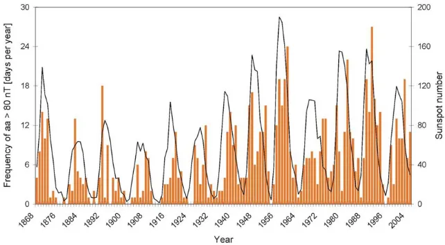
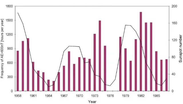
Fig. 1 it is also seen an overall increase in strong geomagnetic activity since the 1900’s, with a partial minimum around 1965. Although the time-range of Dst and AE series is not long enough, this partial minimumcan also be deduced formFigs. 2 and 3.
Figure 1. Frequency in days per year with aa>80 nT together with the sunspot number (black line) during the period 1868–2005.
Figure 3. Frequency in hours per year with AE > 600 nT together with the sunspot number (black line) during the period 1958–1987 (missing data for years 1976 and 1977).
A partial decrease since the 1990’s is suggested by Figs. 1 and 2 which, together with the 1965 minimum, may be part of a long-term cycle modulating an even longer oscillation.
3. SPACE WEATHER EFFECTS
In order to give a rough assessment of one of the expected effects of strong geomagnetic storms on Earth, we present now an estimate of the current and voltage induced in a long pipeline.
Strong geomagnetic activity levels induce important changes in the electric currents in the ionosphere. These currents produce their own changing magnetic fields, B, which in turn induces an electric field, E. This electric field can be estimated in several ways [14–18]. Here, we consider the case when the magnetic field at the surface of the Earth is known. The electric (or geoelectric) field can be obtained then in the frequency domain from the impedance Z(ω):
Ex(ω) = Z(ω)By(ω) (1) Ey(ω) = −Z(ω)Bx(ω) (2)
assumed to be uniform, Z(ω) results:
Z(ω) =
iωµ
σ (3)
µis the magnetic permeability which in the Earth usually has its free value of 4π×10−7H/m.
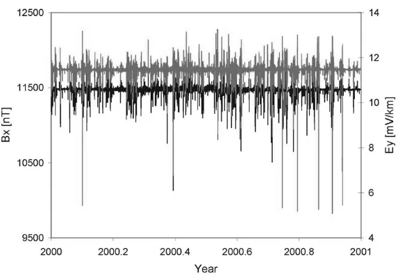
To obtain Ex(ω) and Ey(ω) fromEqs. (1) and (2), the power spectrum of the magnetic field componentsBy(ω) andBx(ω), which are obtained fromhorizontal geomagnetic field records, must be assessed first. In the frequency domain, this power spectrum is multiplied by the surface impedance given by Eq. (3) to obtain the spectrum of the electric field components. An inverse discrete Fourier transform is used then to obtain the electric field variations in the time domain. As an example, Fig. 4 showsBx measured at Sodankyla (67.4◦N, 26.6◦E) for the year 2000 and the resultingEy, both in the time domain.
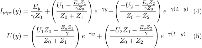
The current and voltage induced in a pipeline, Ipipe and U respectively, can be obtained by using the analogy between pipelines and transmission lines adopted by Boteler and Cookson [19]. This analogy allows the use of the distributed source transmission line (DSTL) theory first described by Schelkunoff [20]. Pulkkinen et al. [21] present a general method to obtain, with the DSTL theory, the current and voltage for buried pipelines when the geoelectric field, the pipe geometry and the electromagnetic properties of the pipelines are assumed to be known. Here we consider the simple situation of a spatially uniform geoelectric field with harmonic time dependence (eiωt).
Assuming a pipeline parallel to they axis, Ipipe and U result:
Ipipe(y) = Ey γZ0
+
U1−
EyZ1
γZ0
Z0+Z1 e−γy+
−U2−
EyZ2
γZ0
Z0+Z2
e−γ(L−y) (4)
U(y) =
U1Z0−EyZγ 1
Z0+Z1
e−γy+
−U2Z0−EyZγ 2
Z0+Z2
e−γ(L−y) (5)
γ = √ZY is the propagation constant and Y is the admittance per unit length of the pipeline coating. Z0 =
Z/Y is the characteristic impedance, the subindices 1 and 2 denote the beginning and the end of the pipeline, andEy is obtained fromEq. (2).
Figure 4. Horizontal x component of the magnetic field, Bx, (black line) measured at Sodankyla (67.4◦N, 26.6◦E) for the year 2000 and the resulting Ey (gray line) assuming a uniform ground conductivity σ.
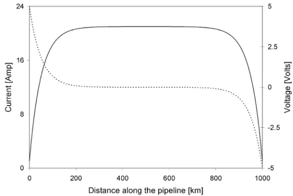
are independent of the pipeline length. The pipeline potentials fall off exponentially with distance fromboth end, and cross through zero in the middle of the pipeline. The current is in phase all along the pipeline and reaches its maximum value in the center of the pipeline.
Even though Eqs. (4) and (5) are the result of great simplifications, the overall effect of changing electric fields on Earth due to strong geomagnetic activity levels can be generalized. For a given geometry and pipeline characteristics, greater Ipipe and U should be expected due to greater geoelectric fields. According to Eqs. (1), (2) and (3), greater fields should be expected if there is an increase in the amplitude of B high frequency components. More power at high frequencies in B spectrum may appear as a result of high magnetic activity levels, that is the occurrence of strong storms and substorms.
4. DISCUSSION AND CONCLUSIONS
Figure 5. The current and voltage induced in a long straight pipeline of 1000 kmlength, Ipipe (solid line) and U (dotted line) respectively.
90 year period) and Suess (∼ 200 year period) cycles, so widely manifested in direct and proxy indicators of different parameters of solar activity [22]. These cycles are two basic modes of long-term solar variability believed to be generated fromthe solar dynamo [23, and references therein]. The last minimum of this cycle occurred in 1905– 1915 [22] so a maximum should be expected around 1990–2010.
Regarding the partial minimum around 1965 (noticed in Figs. 1, 2 and 3), some authors, as Cliver and Ling [1], suggest that it may result froma weak cycle 20 (1964–1976) lying between two strong cycles, 19 and 21. We suggest here that this partial minimum may be the last minimum of the solar Gleissberg cycle (∼80–90 year period), with a maximum around the 1990’s, which would be modulating the much stronger Suess cycle. The previous minimum of the Gleissberg cycle may have occurred around 1880, almost at the time of the Suess cycle last minimum.
REFERENCES
1. Cliver, E. W. and A. G. Ling, “Secular change in geomagnetic indices and the solar open magnetic flux during the first half of the twentieth century,”J. Geophys. Res., Vol. 107, 1303, 2002. 2. Kane, R. P., “Quasi-biennial and quasi-triennial oscillations in
geomagnetic activity indices,” Ann. Geophysicae, Vol. 15, 1581– 1594, 1997.
3. Kane, R. P., “Evolutions of various solar indices around sunspot maximum and sunspot minimum years,” Ann. Geophysicae, Vol. 20, 741–755, 2002.
4. Lockwood, M., R. Stamper, and M. N. Wild, “A doubling of the sun’s coronal magnetic field during the last 100 years,” Nature, Vol. 399, 437–439, 1999.
5. Rangarajan, G. K. and L. M. Barreto, “Long termvariability in solar wind velocity and IMF intensity and the relationship between solar wind parameters & geomagnetic activity,” Earth Planets Space, Vol. 52, 121–132, 2000.
6. Rangarajan, G. K. and T. Iyemori, “Time variations of geomagnetic activity indices Kp and Ap: An update,” Ann. Geophysicae, Vol. 15, 1271–1290, 1997.
7. Rouillard, A. P., M. Lockwood, and I. Finch, “Centennial changes in the solar wind speed and in the open solar flux,” J. Geophy. Res., Vol. 112, A05103, 2007.
8. Russell, C. T., “On the possibility of deducing interplanetary and solar parameters from geomagnetic records,” Solar Physics, Vol. 42, 259–269, 1975.
9. Vennerstrom, S., “Long-term rise in geomagnetic activity — A close connection between quiet days and storms,” Geophys. Res. Lett., Vol. 27, 69–72, 2000.
10. Mayaud, P. N., “Derivation, meaning, and use of geomagnetic indices,” Geophysical Monograph 22, American Geophysical Union, Washington D.C., 1980.
11. Pulkkinen, A., “Geomagnetic induction during highly disturbed space weather conditions: Studies of ground effects,” Academic Dissertation in physics, Contribution 42, 78, Finnish Meteorolog-ical Institute, Helsinki, Finland, 2003.
J. Geophys. Res., Vol. 102, 14189–14198, 1997.
14. Thomson, D. and J. Weaver, “The complex image approximation for induction in a multilayered Earth,”J. Geophys. Res., Vol. 80, 123–129, 1975.
15. Pirjola, R. and A. Viljanen, “Complex image method for calculating electric and magnetic fields produced by an auroral electrojet of finite length,”Ann. Geophysicae, Vol. 16, 1434–1444, 1998.
16. Gummow, R. A. and P. Eng, “GIC effects on pipeline corrosion and corrosion control systems,” J. Atmos. Solar Terr. Phys., Vol. 64, 1755–1764, 2002.
17. Sheherd, S. G. and F. Shubitidze, “Method of auxiliary sources for calculating the magnetic and electric fields induced in a layerd Earth,”J. Atmos. Solar Terr. Phys., Vol. 65, 1151–1160, 2003. 18. Viljanen, A., A. Pulkkinen, O. Amm, R. Pirjola, T. Korja, and
BEAR Working Group, “Fast computation of the geoelectric field using the method of elementary current systems and planar Earth models,” Ann. Geophysicae, Vol. 22, 101–113, 2004.
19. Boteler, D. and M. J. Cookson, “Telluric currents and their affects on pipelines in the Cook Strait region of New Zealand,”Materials Performance, Vol. 28, 27–32, 1986.
20. Schelkunoff, S. A., Electromagnetic Waves, 530, Van Nostrand, New York, 1943.
21. Pulkkinen, A., R. Pirjola, D. Boteler, A. Viljanen, and I. Yegerov, “Modelling of space weather effects on pipelines,” J. Appl. Geophys., Vol. 48, 233–256, 2001.
22. Ogurtsov, M. G., Y. A. Nagovitsyn, G. E. Kocharov, and H. Jungner, “Long-period cycles of the Sun’s activity recorded in direct solar data and proxies,” Solar Physics, Vol. 211, 371–394, 2002.
23. De Jager, C., “Solar forcing of climate. 1: Solar variability,”Space Science Review, Vol. 120, 197–241, 2005.
24. Clilverd, M.A., T. D. G. Clark, E. Clarke, H. Rishbeth, and T. Ulich, “The causes of long-termchanges in the aa index,” J. Geophys. Res., Vol. 107, 2002.