Simulating and Optimizing the Response of a Sine Wave Finite state Machine with Timestamp Simulation Using Simulink

(1)

International Journal of Research (IJR)

e-ISSN: 2348-6848, p- ISSN: 2348-795X Volume 2, Issue 06, June 2015

Available at http://internationaljournalofresearch.org

Simulating and Optimizing the Response of a Sine Wave Finite

state Machine with Timestamp Simulation Using Simulink

Kalpna

1

_{& Mr. Amit Varma}

2

1

_{M. Tech scholar, SGI, Samalkha, Haryana}

2

_{Assistant Professor, Computer Science deptt, SGI Samlkha}

ABSTRACT –

Objective - we have been using sine wave functions from our high school calculus.

Simulation is a integral part of anyone’s life now. We will program in simulink to see how can we simulate a sine wave and obtain a optimized wave. Also we will see how can we change the initial conditions of our parameters in simulation on the run. Secondly we will build a finite state machine that will show a tradeoff between position and velocity using sine wave. It is encountered with many usual problems. We will fix those problems using simulation in simulink at small intervals of time.

CHAPTER – 1

INTRODUCTION

1.Finite State System

An FSM can be represented by a state transition diagram, a directed graph whose vertices correspond to the states of the machine and whose edges correspond to the state transitions; each edge is labeled with the input and output associated with the transition. Suppose that the machine is currently in state 1. Upon input b, the machine moves to states 2 and output 1. Equivalently, an FSM can be represented by a state table with one row for each state and one column for each input symbol (Gillespie, 2008). For a combination of a present state and input symbol, the corresponding entry in the table specifies the next state and output. A state machine represents a system as a set of states, the transitions between them, along with the associated inputs and outputs. So, a state machine is a particular conceptualization of a particular sequential circuit. State machines can be used for many other things beyond logic design and computer architecture.

Circuit with memory is a Finite State Machine. Even computers can be viewed as huge FSMs. Design of FSMs Involves: Defining states, Defining transitions between states, Optimization /Minimization. (Hasheim, 2012)

State Diagram

Illustrates the form and function of a state machine. Usually drawn as a bubble-and-arrow diagram. State

A uniquely identifiable set of values measured at various points in a digital system. (Kumar, 2013) Next State

The state to which the state machine makes the next transition, determined by the inputs present when the device is clocked.

Branch

A change from present state to next state.(Kumar, 2013)

Mealy Machine

A state machine that determines its outputs from the present state and from the inputs.

Moore Machine

A state machine that determines its outputs from the present state only. (Singh et. al., 2012)

On a well-drawn state diagram, all possible transitions will be visible, including loops back to the same state. From this diagram it can be deduced that if the present state is State 5, then the previous state was either State 4 or 5 and the next state must be either 5, 6, or 7. .(Singh et. al., 2012)

Moore and Mealy Machines

(2)

International Journal of Research (IJR)

Moore Machine

Outputs are independent of the inputs, i.e. outputs are effectively produced from within the state of the state machine. (Kumar, 2013)

Mealy Machine

Outputs can be determined by the present state alone, or by the present state and the present inputs, i.e. outputs are produced as the machine makes a transition from one state to another. (Aljeaid et. al., 2014)

SIMULATION - The component-based approach is an important design principle in software and systems engineering. In order to document, specify, validate, or verify components, various formalisms that capture behavioral aspects of component interfaces have been proposed. These formalisms capture assumptions on the inputs and their order, and guarantees on the outputs and their order. (Hasheim, 2012) For closed systems (which do not interact with the environment via inputs or outputs),

a natural notion of refinement is given by the simulation preorder. For open systems, which expect inputs and provide outputs, the corresponding notion is given by the alternating simulation preorder. (Ivan et. Al., 2011) Under alternating simulation, an interface A is refined by an interface B if, after any given sequence of inputs and outputs, B accepts all inputs that A accepts, and B provides only outputs that A provides. (Hasheim, 2012) The alternating simulation preorder is a Boolean notion. Interface A either is refined by interface B, or it is not. However, there are various reasons for which the alternating simulation can fail, and one can make quantitative distinctions between these reasons. For instance, if B does not accept an input that A accepts (or provides an output that A does not provide) at every step, then B is more different from A than an interface that makes a mistake once, or at least not as often as B. (Cerny et al., 2000)

CHAPTER - 2

LITERATURE SURVEY -

WORK DONE BY DIFFERENT RESEARCHERS ON FINITE STATE MACHINE AND SIMULATION IN PREVIOUS YEARS

RESEARCHER OBJECTIVE METHODOLOGY RESULT

Stewart Robinson, (1993)

Discusses simulation, its benefits

and the range of manufacturing

issues to which it can be applied.

A case study Improve work

organization and

determine human

resource requirements.

Horta‐Rangel et al. (2008)

The study of

pressure‐volume‐temperature

(PVT) process is necessary to

understand the physical behavior

of materials. This paper seeks to

Software Analysis. This

simulation procedure

allows one in a simple

way to vary the

(3)

International Journal of Research (IJR)

develop a simulation procedure

to predict phase behavior.

characteristics of the

sample. This makes the

computer simulation a

useful tool together

with the experimental

test, in the development

of novel materials.

R.A. Proctor, (1991)

Development in micro

computer software packages is

examined as they impinge on the

area of creative problem solving

in business. I

Computer modeling A review is provided of

different computer aids

to creative problem

solving and an

overview is given of the

different approaches to

management games.

Many of the different

kinds of management

game are amenable to

computerization.

Dolęga et al. (2012)

To enable the correct selection of

the radiofrequency thermal

ablation (RFTA) process

parameters for an individual

patient by applying a

computer modeling of RFTA.

professional package

of FLUX3D to generate

the geometric models

The computational

results show that the

RFTA algorithm is

effective in solving this

practical problem. The

computational results

show that the selection

of the type of electrodes

(4)

International Journal of Research (IJR)

process is as important

as the correct selection

of the process

parameters, i.e. voltage

and frequency.

G. Southern, (1986)

Demonstrates the techniques of

CAPM by means of manual

simulation.

Computer simulation

model

the CAPM system is

presently installed on

the ACT Sirius and the

IBM personal

microcomputers. It

consists of a series of

basic programs and data

files in four modules.

There is wide scope for

using both versions in

degree courses in

mechanical and

production engineering

and production

management.

Brian Leaned, (1993)

Provides an introduction to

simulation, and discusses the use

of a modern simulation

environment.

simulation tools The gap is even further

reduced if the manager

understands something

of simulation

terminology and

methods. simulation is

(5)

International Journal of Research (IJR)

managers in policy

making and decision

making.

McWaters et al. (1994)

Describes how simulations were

executed for all combinations of

eight fabrics and three contact

surfaces, and presents the

experimental results obtained for

similar conditions and fabrics.

Computer simulation

model

Proves the validity of

the computer model by

comparing the

experimental results

with those obtained

by simulation.

Describes how the

computer model could

be used to choose the

optimum diameter of a

fabric feeder picking

roller.

CHAPTER -3

PAPER OBJECTIVES

Finite state machine response is simulated for corresponding sine wave also simulating the working by simulation using Simulink and Mat lab.

Finite state performance is simulated using simulation in Simulink.

CHAPTER – 4

METHODOLOGY

1. Building a simulation interface for sine wave with appropriate multiplexer and integrator using simulink as a tool.

2. Obtaining the curve for sine wave

3. Varying parameters of simulator on the go. 4. Generating a chart as output of the integrator 5. Designing a state flow structure in the chart

using 3 different states.

6. Designing the tradeoff between 2 basic parameters in the chart.

7. Analyzing the output of finite state machine 8. Output showed when position symbol

becomes positive output does not go to 1. 9. This is called simulation overstepping the

critical time instant.

10. Removing the problem using simulink 11. Obtaining the output curve again at different

small intervals of time.

(6)

International Journal of Research (IJR)

CHAPTER – 5

RESULT AND CONCLUSION

1. Here we have build a model for simulation of continuous sine wave. We are studying how a sine function respnds when simulated in simulink. Structure is shown in figure 2

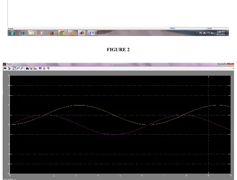
2. When we run this model for time t = 10 units we get the output shown in figure 3

3. Here yellow curve = Velocity sine wave 4. pink curve = Position waveform (Integral

form of velocity sine wave).

5. Now here is an error. Position wave which is obtained by integrating velocity sine wave is starting from point zero.

6. We know integral of sine starts from -1 rather than 0.

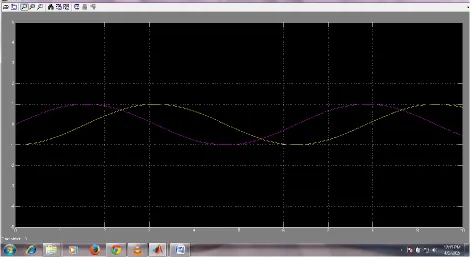
7. We can model this error by using simulink. Which gives the corrected output as shown in figure 4

8. Figure 4 shows Position waveform starting from -1 rather then 0.

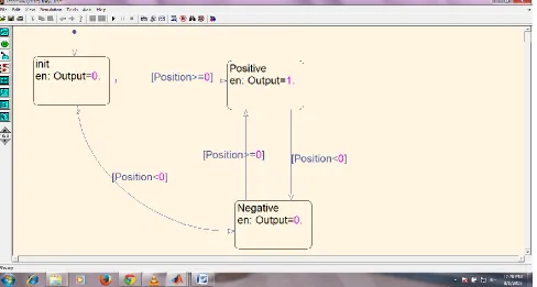
9. Using the existing system shown in figure f1 we will now build a velocity – position finite state machine and chart as shown in figure 5 and 6

10. Figure 5 shows Model for implementing position – velocity finite state machine

11. Figure 6 shows Finite state chart used in the model shown in figure f4

12. Now when we run the above velocity position finite state machine for time units t = 10.0 we get the output shown in figure 7

CHAPTER -6 REFERENCES

[1.]Aljeaid et al., 2014, Modelling and Simulation of a Biometric Identity-Based Cryptography, International Journal of Advanced Research in Artificial Intelligence, Vol. 3, No.10.

[2.]Amr Hasheim , Simulation of Radial Variation of Neutral Atoms on Edge Plasma of Small Size Divertor Tokamak, Bekheit, Journal of Modern Physics, 2012, 3, 145-150 February 2012

[3.]Brian Leaned, (1993) "A Guide to Computer‐based Simulation", Industrial Management & Data Systems, Vol. 93 Iss: 4, pp.8 – 10

[4.]Cerny,(2009) "Comparison between continuous and discrete frequency domain solution methods for structural steady state calculations with the finite element method", COMPEL - The international journal for computation and mathematics in electrical and electronic engineering, Vol. 28 Iss: 4, pp.1068 – 1080

[5.]Dagmara M. Dołęga, Jerzy Barglik, (2012) "Computer modeling and simulation of radiofrequency thermal ablation", COMPEL - The international journal for computation and mathematics in electrical and electronic engineering, Vol. 31 Iss: 4, pp.1087 – 1095

[6.]G. Southern, (1986) "Teaching the Techniques of Computer Aided Production Management and Simulation Modelling", International Journal of Operations & Production Management, Vol. 6 Iss: 1, pp.15 – 24

[7.]Gillespie, Implementing the Stochastic Simulation Algorithm, Journal of Statistical Software, April 2008, Volume 25, Issue 12

(7)

International Journal of Research (IJR)

Journal of Computer Science Issues, Vol. 10, Issue 1, No 1, January 2013

[9.]Ivan et. Al., 2011, Collaborative Systems – Finite State Machines, Informatica Economică, vol. 15, no. 2.

[10.] J.Horta‐Rangel (2008) "Computer simulation of a pressure‐volume‐temperature process", International Journal of Numerical Methods for Heat & Fluid Flow, Vol. 18 Iss: 1, pp.24 – 35

[11.] S.D. McWaters, T.G. Clapp, J.W. Eischen, (1994) "Automated Apparel Processing: Computer Simulation of Fabric Deformation for the Design of Equipment", International Journal

of Clothing Science and Technology, Vol. 6 Iss: 5, pp.30 – 38

[12.] R.A. Proctor, (1991) "Can Computers Simulate Managerial Creativity?", Leadership & Organization Development Journal, Vol. 12 Iss: 4, pp.13 – 16

[13.] Singh et. al.,2012, Finite State Testing and Syntax Testing, International Journal of Computers & Technology, Volume 3. No. 1

[14.] Stewart Robinson, (1993) "The Application

of Computer Simulation in

Manufacturing", Integrated Manufacturing Systems, Vol. 4 Iss: 4, pp.18 – 23

FIGURES USED IN THE PAPER

CONDITION/STATE STATE 1 STATE 2 … STATE i … STATE p

CONDITION 1

CONDITION 2 STATE 3

….

CONDITION j STATE K

….

(8)

International Journal of Research (IJR)

FIGURE 1 - The state diagram for a finite state machine

FIGURE 2

(9)

International Journal of Research (IJR)

FIGURE 4

(10)

International Journal of Research (IJR)

FIGURE 6