Color Separation for Image Segmentation

Scholarship@Western

Scholarship@Western

Electronic Thesis and Dissertation Repository

12-16-2013 12:00 AM

Color Separation for Image Segmentation

Color Separation for Image Segmentation

Meng Tang

The University of Western Ontario

Supervisor Yuri Boykov

The University of Western Ontario Graduate Program in Computer Science

A thesis submitted in partial fulfillment of the requirements for the degree in Master of Science © Meng Tang 2013

Follow this and additional works at: https://ir.lib.uwo.ca/etd

Part of the Artificial Intelligence and Robotics Commons

Recommended Citation Recommended Citation

Tang, Meng, "Color Separation for Image Segmentation" (2013). Electronic Thesis and Dissertation Repository. 1834.

https://ir.lib.uwo.ca/etd/1834

This Dissertation/Thesis is brought to you for free and open access by Scholarship@Western. It has been accepted for inclusion in Electronic Thesis and Dissertation Repository by an authorized administrator of

(Thesis format: Monograph)

by

Meng Tang

Graduate Program in Computer Science

A thesis submitted in partial fulfillment

of the requirements for the degree of

Masters of Science

The School of Graduate and Postdoctoral Studies

The University of Western Ontario

London, Ontario, Canada

c

Image segmentation is a fundamental problem in computer vision that has drawn intensive

research attention during the past few decades, resulting in a variety of segmentation

algo-rithms. Segmentation is often formulated as a Markov random field (MRF) and the solution

corresponding to the maximum a posteriori probability (MAP) is found using energy

minimiza-tion framework. Many standard segmentaminimiza-tion techniques rely on foreground and background

appearance models given a priori. In this case the corresponding energy can be efficiently

op-timized globally. If the appearance models are not known, the energy becomes NP-hard, and

many methods resort to iterative schemes that jointly optimize appearance and segmentation.

Such algorithms can only guarantee local minimum.

Here we propose a new energy term explicitly measuring the L1 distance between object and

background appearance models that can be globally maximized in one graph cut. Our method

directly tries to minimize the appearance overlap between the segments. We show that in many

applications including interactive segmentation, shape matching, segmentation from stereo

pairs and saliency segmentation our simple term makes NP-hard segmentation functionals

un-necessary and renders good segmentation performance both qualitatively and quantitatively.

Keywords: Image Segmentation, Appearance Model, Markov Random Fields, Color

Sep-aration, Submodular Function Minimization, Pesudo-boolean Function

Section 1.3inChapter 1is primarliy written by my advisor Dr. Yuri Boykov. The motivation

of this work is brought forward and contribution is summarized. Other parts inChapter 1, 2

and3are based on my own summary of related work.

Chapter 4is collaboration work with Dr. Lena Gorelick. I programmed the code for all

ap-plications and wroteChapter 5by my self. Dr. Olga Veksler gave me the valuable suggestion

of comparing different color separation terms. The idea of combining color separation term

with template shape prior is from Dr. Yuri Boykov, which leads to template shape matching

application inSection 5.2.

I would like to thank my advisor Dr. Yuri Boykov and informal co-advisor Dr. Olga Veksler.

When I need help in my research, they are always there, listening to my ideas, discussing with

me and sparkling new ideas. They really care about my research and help me grow. I still

re-member the first meeting with Dr. Yuri Boykov and Dr. Olga Veksler when I had a small idea

about dynamic graph cut and amazingly they quickly set up a meeting with me. They were

willing to listen to and develop my idea even though I was just a first year graduate student

at that time. Working with them is a lot of fun, highly efficient and I learnt how to do real

research from scratch. Especially, I gained a sense of what is important research from them. I

am fortunate to have them as advisors.

Thank you Dr. Lena Gorelick for helping me with my research project. I bothered you too

many times and each time you patiently answered my questions and even helped me

trou-bleshoot technical problem of my project. Thank you Dr. Andrew Delong, a former member

of the computer vision group, for proving data used in your label cost paper when I requested.

I appreciate the hard-working of the thesis committee members, including Dr. Roberto

Solis-Oba, Dr. Stephen Watt and Dr. Hristo Sendov. Their advices help me a lot in presenting this

work.

I would also like to thank other members of the computer vision group at Western

Univer-sity including Liqun Liu, Xuefeng Chang, Igor Milevskiy and Yuchen Zhong. Even though

they have different research projects from me, I also benefit from their outstanding research

progress and they provided great pieces of advice on my research. Life without these lovely

friends would be boring.

Last but not least, I would like to thank my parents and sister who support my study in Canada

and give me this wonderful life I’ve ever experienced.

Abstract ii

Co-Authorship Statement iii

Acknowlegements iv

List of Figures vii

List of Tables x

1 Introduction 1

1.1 Markov Random Fields: Modeling and Inference . . . 2

1.2 Markov Random Fields for Image Segmentation . . . 6

1.3 Motivation of Color Separation Term for Image Segmentation . . . 7

1.4 Contribution of the Thesis . . . 13

1.5 Outline of the Thesis . . . 14

2 Overview of Appearance Models 15 2.1 Histogram . . . 15

2.2 Non-parametric Density Estimation . . . 16

2.3 Gaussian Mixture Model . . . 17

3 Related Work 20 3.1 GrabCut . . . 20

3.2 Branch-and-Mincut . . . 22

3.3 Dual Decomposition . . . 23

3.4 Active Contour . . . 23

4 Minimizing Appearance Overlap in One-cut 25 4.1 L1Color Separation Term . . . 25

4.2 Minimizing Higher-order Pseudo-boolean Function . . . 27

5 Applications 31

5.1 Interactive segmentation . . . 31

5.1.1 Binary segmentation with bounding box . . . 31

5.1.2 Comparison of Appearance Overlap Terms . . . 38

5.1.3 Interactive Segmentation with Seeds . . . 40

5.2 Template Shape Matching . . . 41

5.3 Salient object segmentation . . . 43

5.4 Foreground Segmentation from Stereo . . . 45

6 Future Work and Conclusion 48 6.1 Color Separation Term for GMM Appearance Model . . . 48

6.2 Color Separation Term with Supermodular Term . . . 48

6.3 Feature Separation Term for Multi-label Inference . . . 50

6.4 Conclusion . . . 51

Bibliography 52

A Proofs of Theorems 58

Curriculum Vitae 59

1.1 Markov Property: The state of the black node is conditionally independent of

all the white nodes, given the states of the gray nodes. This is called the Markov

property. . . 2

1.2 Hidden Markov Model on a 4-connected graph. The upper layer represents

observed value of nodes and the lower layer represents hidden state variables

of nodes. . . 3

1.3 Take LP relaxation of the original energy with discrete variables and maximize

the lower bound. . . 5

1.4 Graph Cut for Interactive Segmentation: (top-left) User specified seeds denoted

by blue and red pixels, (top-right) Graph with pixels as nodes and S, T

termi-nals, (bottom-left) Graph with t-links and n-links, (bottom-right) s/t mincut.

[Image credit: Yuri Boykov] . . . 8

1.5 Interactive image segmentation: user provided strokes (Left) and result (right). . 9

1.6 If we only optimize the first two terms in (1.15) and restrict the foreground to

be a rectangle, we can get a rough bounding box of foreground and background

in sliding-window fashion. The foreground is indicated by red box. . . 10

1.7 Color separation gives segments with low entropy. . . 10

1.8 Energy (1.15): volume balancing (a) and Jensen-Shannon color separation

terms (b). OurL1color separation term (c). . . 11

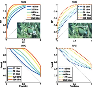
1.9 ROC curves of thresholding log likelihood ratios with different number of color

bins used in color histogram . . . 13

2.1 Binning in RGB color space1 . . . 16

2.2 Window size is fixed for Parzen window (left) and number of neighboring

points is fixed fork-NN(right). Window size or number of neighboring points should be chosen properly to get a good density estimation. c⃝Olga Veksler. . . 17

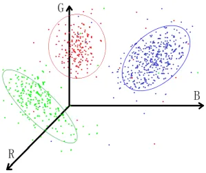
2.3 Gaussian Mixture Model in RGB color space. In this example we have three

Gaussian mixture components highlighted by three ellipses. . . 19

3.2 Branch-and-Mincut [40] can find smaller global energy while GrabCut gets

stuck in local minima with larger energy. . . 22

3.3 (top row) Intensity-based segmentation of Zebra at each iteration. (bottom row)

Corresponding intensity distributions of Zebra and its background. Pin and

Poutare intensity distributions of regions inside and outside the contour. [45] . 24 4.1 Graph construction forEL1 in one color bin: nodesv1,v2, . . . ,vnk corresponding

to the pixels in bin k are connected to the auxiliary nodeAk using undirected

links. The capacity of these links is the weight of appearance overlap termβ >0. 26 4.2 Overall graph construction for energy withL1 color separation term. . . 26

4.3 Our graph for minimizing pseudo-boolean function (4.3) . . . 27

4.4 Graph for minimizing pseudo-boolean function (4.3) by Kohli et al. [30, 31] . . 29

4.5 Appearance overlap terms based on different metrics: L1 norm, χ2 distance,

Bhattacharyya coefficient and Jensen-Shannon divergence . . . 30

4.6 The original concave function (red) is approximated as a piece-wise linear

function (blue, left) using three truncated components (blue,middle).

Approxi-mation with ten components (blue, right) is already very accurate. . . 30

5.1 Error-rates for different bin resolutions, as in Table 5.1. . . 34

5.2 Example of segmentation results. From left to right: (a) user input, (b)

Grab-Cut [9, 51], (c) Dual Decomposition (DD) [59], (d) our One-Grab-Cut. For these

examples we used 163 _{bins. . . 35}

5.3 Example of segmentation results obtained with our One-Cut. For these

exam-ples we used 1283bins. . . 36

5.4 Example of segmentation results obtained with our One-Cut. For these

exam-ples we used 163_{bins. . . 37}

5.5 Error rates and running time comparison of different appearance overlap terms. 38

5.6 Left: Truncated appearance overlap termD_LT

1 for a bink. Right: Segmentation error rate as a function of parametertinDT_L

1. Best results are achieved fort=1 (no truncation). . . 39

5.7 Interactive segmentation with seeds . . . 40

5.8 Template shape matching examples, from left to right: Original images,

con-trast sensitive edge weights, shape matching results without and with the

ap-pearance overlap penalty. Input shape templates are shown as contours around

the resulting segmentation. . . 41

5.10 Different saliency maps . . . 43

5.11 Saliency segmentation results reported for dataset [1]: Precison-Recall and

F-measure bars forE3(S),E4(S) are compared to FT[1], CA[24], LC[64], HC[19]

and RC[19]. . . 44

5.12 Saliency segmentation examples: (a) Original image, (b) Saliency map from

[49] with bright intensity denoting high saliency, (c-d) Graph cut segmentation

without and with appearance overlap penalty term, (e) Ground truth. . . 46

5.13 Foreground segmentation from stereo pair (a) One of input stereo images, (b)

Segmentation result when optimizing energyE5(S) (5.12) (c) Refine (b) with

EM (d) Segmentation with color separation augmented energyE6(S) (5.14). . . 47

6.1 Color separation term for Gaussian Mixture Model. . . 49

6.2 Combine color separation term with FTR for volume balancing term. . . 50

4.1 Cut costs corresponding to four possible label assignments to the binary

auxil-iary nodesA1

k andA

0

k. The optimal cut must choose the minimum of the above

costs, thus minimizing (4.3). . . 28

5.1 Error rates and mean runtime for GrabCut [9, 51], Dual Decomposition (DD)

[59], and our method, denoted byOne-Cut. . . 33 5.2 Template shape matching results with or without color separation term: TP, FP,

misclassified pixels, and mean running time. . . 42

Introduction

Image segmentation is the problem of partitioning the image into several segments. Pixels

in the same segment should have similar characteristics, such as intensity, color, texture, etc.

On the other hand, pixels in different segments should have distinct characteristic of the same

measure. Sometimes image segmentation is a goal in itself. A user might want to segment an

object from an image to paste in another image. Most often, segmentation is needed for other

vision or medical imaging applications. For example, for medical diagnosis and prognosis of

cancer patients, one often needs to accurately measure the tumor volume, which first requires

segmenting a tumor from a medical MRF volume. Another application where image

segmen-tation is useful is object detection. Segmensegmen-tation is useful for feature extraction [53] and to

limit the number of image patches to examine for a possible presence of an object [39].

Simply stated, image segmentation can be viewed as a labeling problem where each pixel is

assigned a label. There are two labels for segmentation into two regions and multiple labels for

segmentation into multiple regions.

Image segmentation can be performed in a supervised or unsupervised fashion. In unsupervised

segmentation, no user assistance is available and typically, no additional knowledge about the

scene contents is assumed. In supervised segmentation, user specifies either a bounding box

containing the object of interest, or so called object and background ”seeds”, indicating some

pixels that belong to the object and background, respectively. We may have prior knowledge

of segments such as volume ratio of the segments, target distribution of segments learned from

a training dataset or shape of the segments. The prior knowledge or user interaction is often

incorporated into image segmentation algorithms.

Over the past few decades, numerous algorithms have been developed for image segmentation.

Commonly used methods include live-wire [46], deformable models [28], normalized-cut [52],

level sets [20, 43], graph cut [12, 14], etc. The focus of this thesis is energy minimization

meth-ods for image segmentation. We use the popular and well-known s-t mincut for optimization.

1.1

Markov Random Fields: Modeling and Inference

Markov Random Field (MRF) [10, 33] is a graphical model of joint probabilistic distribution

on a set of random variables which are inter-dependent, and their dependences can be modeled

with a graph. MRFs have been applied to a wide range of problems in computer vision such

as image segmentation, image restoration, 3D reconstruction and image & video Synthesis

[21, 38]. We often express a Markov Random Field as a graphG = {V,E}whereV is the set of vertexes andEis the set of edges. MRF satifisfies the Markov property that the state of one

node is independent of all other nodes given the states of its neighboring nodes. For example,

in Fig. 1.1, the state of the black node, when conditioned on the four gray neighboring nodes,

is independent of all the other graph nodes.

The simplest Markov model- Markov Chain- is defined on a sequence of random variables

X = {x1,x2, ...}over time where the conditional probability of variable xi only depends onxi−1:

P(xi|xi−1,xi−2, ...,x1)=P(xi|xi−1). (1.1)

A MRF can be seen as extension of a Markov Chain with higher-order clique (minimum set

of connected nodes) and larger connectivity dimension. We often treat each pixel as one node

and use 4 or 8 neighboring system as graph for Markov model in computer vision.

Figure 1.1: Markov Property: The state of the black node is conditionally independent of all the white nodes, given the states of the gray nodes. This is called the Markov property.

A Markov Random Field encodes the long-range correlation between states of variables by

simply connecting nodes to a few neighboring nodes. By doing this we avoid densely

con-nected graph which needs computationally expensive inference algorithms and yet capture the

essential dependences between the pixels.

Figure 1.2: Hidden Markov Model on a 4-connected graph. The upper layer represents ob-served value of nodes and the lower layer represents hidden state variables of nodes.

variables byXand observations of nodes byZfor HMM. Applying Bayes’ theorem, we have

P(X|Z)∝ P(Z|X) P(X). (1.2)

For the likelihoodP(Z |X), each observed datazi only depends on the state of hidden variable

xi. The distributionP(X) is assumed to follow the Markov property.

The above posterior MRF is often expressed as energy by taking the log:

P(X |Z)= 1

Zexp (−E(X|Z)), (1.3)

E(X |Z)=∑

c∈C

θc(X)+

∑

i

ϕ(xi,zi), (1.4)

whereZis the normalization factor. HereCis the set of cliques.

Eachθc(X) is called a clique potential. A clique contains fully connected subsets of nodes in

the graph. The degree of a clique is the number of nodes in the clique. If the degree of cliques

is more than three, we treat the MRF as high-order MRF and the corresponding optimization

problem is often more challenging. A typical high-order clique is the term defined over number

of pixels in segments, for example, term penalizing deviation of segment size from target size.

The simplest cliques include one-degree clique and two-degree clique which get involved only

one node or two nodes respectively in the clique.

its neighboring nodes in the graph given the observed data Z, so the clique potential is of the formθc(X,Z) rather thanθc(X). A CRF can be seen as a MRF globally conditioned on the

observation. One application of CRF is binary image segmentation with edge-contrast sensitive

smoothness term which will be explained later.

Inferrence of posterior MRF is a Maximum A Posteriori (MAP) problem :

X =argmaxP(X |Z) (1.5)

or equivalently we can minimize the energyE(X|Z).

The most commonly used MRF energy consists of an unary term and a pairwise term:

E(X |Z)=∑

i∈V

ϕi(xi,zi)+

∑

(i,j)∈E

θi j(xi,xj), (1.6)

where variablexitakes value from label setLandziis the observation of nodei.

Generally, the MAP-MRF energy (1.6) optimization is NP-hard, even for binary case where

the variablexi can only take label 0 or 1. In the binary case, if the pairwise potential satisfies:

θi j(0,0)+θi j(1,1)≤θi j(0,1)+θi j(1,0),∀(i, j), (1.7)

then the energy (1.6) is submodular and can be optimized with a graph cut [36]. Intuitively

speaking, a submodular energy encourages nearby pixels to have same labels. Boykov and

Kolmogorov [14] have developed a min-cut/max-flow algorithm that is particularly efficient in

practice for graphs of small connectivity, that naturally arise in image segmentation problems.

MRF optimization methods have two important groups: those in discrete and those in

contin-uous domains. Graph cut is a popular discrete domain optimization method that can optimize

submodular energy functions. For binary MRF optimization of submodular energy, graph cut

gives global optimal solutions in polynomial time. For multi-label MRF when the pairwise

ter-mθi j(xi,xj) is metric or semi-metric, graph cut can find approximate solution by move-making

algorithm converges when there is no furtherα−βswap (orα-expansion) move that decreases the energy.

Belief propagation [22, 48, 54, 63] is another important early discrete optimization method

for energy (1.6). BP can be seen as re-parameterization of the original energy and gives exact

solution on trees, but it gives local minima if there are loops in the graph and may not even

converge. BP usually returns an energy which is worse than that of a graph cut.

In the continues optimization domain [2, 18, 29, 37], the MRF optimization problem is written

as an integer program (IP). Denote the set of possible labels as L, by relaxing the integration constraints of the integer program, the IP can be further written as the following Linear

Pro-gram (LP) and solved by LP solver such as interior point methods. However, the solution of LP

needs to be rounded and can be far from the optimal solution of IP and LP solver is relatively

slow in practice.

min ∑

i∈V,xi∈L

ui(xi)ϕi(xi)+

∑

(i,j)∈E,xi,xj∈L

ui j(xi,xj)ϕi j(xi,xj) (1.8)

subject to: _∑

xi,xj∈L

ui j(xi,xj)= 1, (1.9)

∑

xi∈L

ui j(xi,xj)=uj(xj), (1.10)

ui j(xi,xj),ui(xi)∈[0,1]. (1.11)

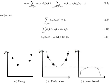
(a) Energy (b) LP relaxation (c) Lower bound

Figure 1.3: Take LP relaxation of the original energy with discrete variables and maximize the lower bound.

relax-ation (Fig. 1.3). TRW represents the graph as convex combinrelax-ation of trees. The summrelax-ation

of minimum of trees gives lower bound of the original energy. The two major steps of TRW

include performing BP on trees and averaging nodes selected by particular scheme. TRW

iter-ates between the two steps until convergence, which gives local maximum of lower bound. A

nice property of TRW-S [34] is that the lower bound never decreases.

1.2

Markov Random Fields for Image Segmentation

S-t maxflow/mincut is first used by Greig et al. [26] as optimization algorithm for

comput-er vision and image processing. Thcomput-ere it is used for the task of binary image reconstruction

from noisy images. Then Boykov and Jolly first employed graph cut for image segmentation

[11, 12, 13, 14]. Bellow we show an example of graph cut for binary interactive image

seg-mentation.

We denotesp ∈ {0,1}as binary indicator variables for pixel p, 1 for foreground and 0 for

back-ground. The most commonly used single-variable potential is log-likelihood term ln Pr(Ip|θsp)

for each pixel p, where θ1 and θ0 are fixed foreground and background appearance models, usually based on color distributions. Ip is the color of pixel p. In the case of interactive

seg-mentation, we can estimate the initial appearance model through user input strokes. Sometimes

the appearance model of foreground and background are known a priori, for example from a

training set. Commonly used pairwise potential is edge-contrast sensitive smoothness

penal-ty. The higher the intensity contrast between two adjacent pixels, the smaller the smoothness

penalty.

The basic object segmentation energy [12, 57] combines boundary length regularization ∂S

with log-likelihood term

E(S|θ1, θ0) = −∑

p∈Ω

ln Pr(Ip|θsp) + |∂S| (1.12)

whereΩis the set of all image pixels andS is the set of foreground pixels labelled assp = 1.

The most commonly used boundary length regularization term is |∂S| = ∑_{p,q}∈Nωpq|sp− sq|

andNis the set of all pairs of neighboring pixels. Ifωpqis constant, then the smoothness term is

data independent and the model is MRF. Ifωpqis edge-contrast sensitive, then the smoothness

term depends on the observed data and the model becomes a CRF. The log-likelihood term,

or data term is a unary term, and the smoothness term is a pairwise term. A real example of

Example: Interactive image segmentation with graph cut (Fig. 1.4)

1. The user specifies hard-constrained pixels that have to be segmented as foreground or

background. For example, the user can put strokes on object and background. We can

estimate foreground and background appearance model (color histogram) accrording to

the strokes.

2. A four or eight connected graph is constructed with each node representing each pixel

and there are two additional terminal nodes in the graph: source node S and sink node

T.

3. Then we connect nodes in the graph through links. The links between pixels and

ter-minals are denoted by t-links and links between pixels themselves are denoted by

n-links. The hard-constrained pixels are linked to terminal nodes S or T with infinity edge weights. Other pixels are linked to terminal nodes through soft-constrain t-link,

the weight of which will be explained later. One way of setting soft-constrain t-link is

through appearance model of foreground and background.

4. Adjacent pixels in neighboring system are connected through n-links. The weight of the

smoothness term can be edge-contrast sensitive.

5. After the graph is constructed, we can use any available maxflow/mincut optimization

algorithm and get the cut of minimum weight. The min cut specifies whether the pixels

belong to foreground and background.

1.3

Motivation of Color Separation Term for Image

Segmen-tation

Appearance models are critical for many image segmentation algorithms. One important

prac-tical advantage of this basic energy is that there are efficient methods for their global

minimiza-tion using graph cuts [14] or continuous relaxaminimiza-tions [16, 50].

In many applications the appearance models may not be known a priori. Some well-known approaches to segmentation [17, 51, 66] consider model parameters as extra optimization

vari-ables in their segmentation energies. E.g.,

E(S, θ1, θ0) = −∑

p∈Ω

Figure 1.4: Graph Cut for Interactive Segmentation: (top-left) User specified seeds denoted by blue and red pixels, (top-right) Graph with pixels as nodes and S, T terminals, (bottom-left) Graph with t-links and n-links, (bottom-right) s/t mincut. [Image credit: Yuri Boykov]

which is known to be NP-hard for optimization [59], is used for interactive segmentation in

GrabCut [9, 51] where initial appearance models θ1_, θ0 _{are computed from a given bounding}

box. The most common approximation technique for minimizing (1.13) is a block-coordinate

descent [51] alternating the following two steps. First, they fix model parameters θ1_, θ0 _and

optimize overS, e.g. using a graph cut algorithm for energy (1.12) as in [12]. Second, they fix segmentation S and then optimize over model parameters θ1 _{and θ}0_{. Two well-known}

alternatives, dual decomposition [59] and branch-and-mincut [40], sometimes find a global minimum of energy (1.13), but these methods are too slow in practice. Please refer toChapter

3for detailed description on GrabCut,dual decompositionandbranch-and-mincut.

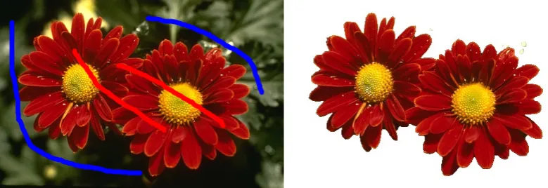
Figure 1.5: Interactive image segmentation: user provided strokes (Left) and result (right).

histograms, we can rewrite (1.13) as :

E(S, θ1, θ0) = −∑

sp=1

ln Pr(Ip|θ1) −

∑

sp=0

ln Pr(Ip|θ0) + |∂S|

= −∑

k

nS_k lnθ1_k −∑

k

nS_k¯lnθ0_k + |∂S|

= −|S|∑

k

θS k lnθ

1

k − |S¯|

∑

k

θ_S¯

k lnθ

0

k + |∂S|

= |S| ·H(θS|θ1)+|S¯| ·H(θS¯|θ0)+|∂S|, (1.14) where nS_k is the number of pixels inkth color bin in foreground and nS_k¯ in background. Here

θS _{and θ}S¯ _{are histograms inside objectS and background ¯S = Ω\S. H(θ}S_|θ1_{) and H(θ}S¯_|θ0₎

are cross entropies of probability distributions. According to well-known cross entropy

in-equality H(θS|θ1₎ ≥ _H(θS_{) where H(}·_{) is the entropyfunctional for probability distributions,}

minimization of (1.13) is equivalent to minimization of energy

E(S) = |S| ·H(θS)+|S¯| ·H(θS¯)+|∂S| (1.15) that depends onS only. Interestingly, the global minimum of segmentation energy (1.15) does not depend on the initial color models provided by the user. Thus, the interactivity of GrabCut

algorithm is primarily due to the fact that its solution is a local minimum of (1.15) sensitive to

the initial bounding box.

If we ignore the smoothness term and use a sliding window to find the bounding box that

minimizes energy (1.15), we would get a box that splits the object of distinct appearance from

the background in the image. See Fig. 1.6 for example. We used integral image [60] which is

originally used for face detection to help accelerate the optimization.

Figure 1.6: If we only optimize the first two terms in (1.15) and restrict the foreground to be a rectangle, we can get a rough bounding box of foreground and background in sliding-window fashion. The foreground is indicated by red box.

terms of this energy prefer segments with more peaked color distributions that give lower

en-tropy. Intuitively, this should also imply that the optimal foreground and background

distribu-tions have a small overlap. For example, consider a simple case of black-&-white image when

color histogramsθ1 andθ0 have only two bins (Fig. 1.7). Clearly, the lowest value (zero) for the entropy terms in (1.15) is achieved when black and white pixels are completely separated

between the segments, e.g. all white pixels are inside the object and all black pixels are inside

the background.

(a) High entropy example (b) Low entropy example

Figure 1.7: Color separation gives segments with low entropy.

The intuitive observation that separating pixels of the same color into different segments

We can further rewrite energy (1.15) as:

E(S) = −|S|∑

k

θS k lnθ

S k − |S¯|

∑

k

θ_S¯

k lnθ

¯

S

k + |∂S|

= −∑

k

nS_k lnθS_k −

∑

k

nS_k¯ lnθ_kS¯ + |∂S|

= −∑

k

nS_k ln n

S k

|S| −

∑

k

nS_k¯ln n

¯

S k

|_S¯_| + |∂S| = |S|lnS +|S¯|ln|S¯| −∑

k

(nS_k lnnS_k +n_kS¯ lnnS_k¯) + |∂S| (1.16) So the color separation bias in energy (1.15) is shown by equivalently rewriting its two entropy

terms as

h_Ω(S)−

∑

i

h_Ωi(Si) (1.17)

wherehA(B)=|B|·ln|B|+|A\B|·ln|A\B|is standard Jensen-Shannon (JS) divergence functional

for subsetB ⊂ A. We also use Ωi to denote the set of all pixels in color bini(noteΩ =∪iΩi)

andSi =S∩Ωiis a subset of pixels of coloriinside object segment (noteS = ∪iSi). The plots

for functionsh_Ω(S) and−h_Ωi(Si) are illustrated in Fig.1.8.

GC volume

balancing

term

JS separation

term

Our L

separation

term

S

GC volume

balancing

term

S

S

(a) h_Ω(S) (b) −h_Ωi(Si) (c) −|Si−S¯i|

Figure 1.8: Energy (1.15): volume balancing (a) and Jensen-Shannon color separation terms (b). OurL1color separation term (c).

The first term in (1.17) shows that energies (1.13) or (1.15) implicitly bias image segmentation

to two segments of equal size, see Fig.1.8(a). The remaining terms in (1.17) show bias to color

separation between the segments, see Fig.1.8(b). Note that a similar analysis in [59] is used to

motivate their convex-concave approximation algorithm for energy (1.13).

Relation with Normalized Cuts: The combination of color separation term and volume

bal-ancing term is analogous to Normalized Cuts [52]. In Normalized Cuts, the graph partition

criteria is given by:

Ncut(A, B) = cut(A, B)

Vol(A) +

cut(A, B)

wherecut(A, B) is the sum of weights of connections between groups Aand BandVol(A) is the total weight of the edges originating from groupAandVol(B) is similarly defined. The ter-mcut(A, B) plays a similar role as smoothness term|∂S|that minimizes the boundary length. If there’s only the termcut(A, B) in the energy, then trivial solutions ofA =∅orB= ∅would be global optimal solutions. The volume terms Vol(A) and Vol(B) have the same effects as volume balancing term hereh_Ω(S) that prefers balanced foreground and background. Note that normalized cut does not have a color separation term. The lack of color separation can lead to

significant artifacts in segmentation, where volume balancing plays too much of a role. This

often results in segments that are almost equal in volume, but perceptually not distinct.

Volume balancingh_Ω(S) is the only term in (1.17) and (1.13) that is not submodular and makes optimization difficult. Our observation is that in many applications this volume balancing term

is simply unnecessary [55], see Sections 5.1.3, 5.2-5.3. In other applications we propose to

replace it by other easier to optimize terms.

Moreover, it is known that JS color separation term−h_Ωi(Si) is submodular (any concave

func-tion of cardinality (number of pixels in segment) is submodular [42]. This applies to JS, χ2, Bhattacharyya, and our L1 color separation terms in Figs.1.8, 5.5.), so it can be optimized by

graph cuts [30, 31, 59]. We propose to replace it with a simpler L1 separation term [55] in

Fig.1.8(c). We show that it corresponds to a simpler construction with fewer auxiliary nodes

leading to higher efficiency while capturing the essence of a more general color separation

ter-m. Interestingly, it also gives better color separation effect in practice for some applications,

see Section 5.1.2. A Bhattacharyya gradient flow driven active contour can also maximize the

discrepency between distribution of regions inside and outside the active contour [45], but

op-timization of the level set energy is very slow.

We also observe one practical limitation of block-coordinate approach to (1.13), as in GrabCut

[9, 51], could be due to increased sensitivity to local minima when the number of color bins for

modelsθS andθS¯ is increased, seeSection 3.1, Table 5.1 and Fig.5.1. The reason is that with more color bins, the dimensionality of the histogram gets larger, and there are more local

mini-mums of the energy function. This is because there are more histogram-based color models for

foreground and background that result in a good color separation. In practice, however, finer

bins better capture the information contained in the full dynamic range of color images (8-bit

per channel or more). Our ROC curves show that even a difficult camouflage image in Figure

1.9 has a good separation of intensities between the object and background if larger number of

bins is used. With 163_{bins, however, the overlap between the “fish” and the background is too}

strong making it hard to segment. Since GrabCut algorithm is more likely to get stuck at weak

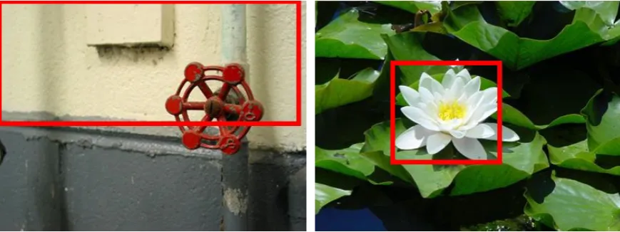
Figure 1.9: Given appearance modelsθo_,θb_{extracted from the ground truth object}/_background

segments (white contour, top-left), we can threshold log-likelihood ratios lnθo(Ip)

θb_(I

p) at each pixel

p and compare the result with the same ground truth segmentation for different thresholds. The corresponding ROC (top-left) curves and RPC curves (bottom-left) show that the color separation between the object and background increases for finer bins. The same procedure is repeated for an arbitrary chosen rectangle within the same image (top-right, bottom-right) with far less pronounced improvement. It is clearly seen that using higher number of bins to represent appearance can help separate objects from the background even in the case of camouflage images.

1.4

Contribution of the Thesis

The contribution of the thesis is summarized as follows:

• We propose a simple energy term penalizingL1measure of appearance overlap between

segments. While it can be seen as a special case of a high-orderlabel consistencyterm introduced by Kohli et al. [30, 31] we propose a simpler construction for our specific

con-straint. Unlike NP-hard multi-label problems discussed in [30, 31], we focus on binary

segmentation where such high-order constraints can be globally minimized. Moreover,

we show that ourL1term works better for separating colors than other concave separators

• We are first to demonstrate fast globally optimal binary segmentation technique explicitly minimizing overlap between un-normalized object/background color histograms. In one

graph cut we get similar or better results at faster running times w.r.t. earlier methods,

e.g. [19, 40, 51, 59].

• We show general usefulness of the proposed appearance overlap penalty by showing different practical applications: binary segmentation, shape matching, etc.

1.5

Outline of the Thesis

The thesis is organized as follows: Chapter 2 is an overview of appearance models for

seg-ments, including non-parametric density estimation such as Parzen window andk-NN density estimation and parametric density estimation Gaussian mixture model. In Chapter 3

realat-ed work of GrabCut, branch-and-mincut, dual decompostion and active contour is analysed and limitations of these approaches are shown. InChapter 4 our proposed L1 color

separa-tion term is introduced, we also explain the relasepara-tionship bettweenL1color separation term and

general color separation term. We show the graph construction for minimizing these color

sep-aration terms. Furthermore we explain the difference of ourL1 color separation term fromPn

Potts model. Chapter 5presents several applications of our color separation term. We apply

the color separation term to segmentation with bounding box or seeds, shape matching with

a simple template and salient object segmentation. Our algorithm based on color separation

term outperforms the state of the art. Chapter 6concludes the thesis by pointing out several

Overview of Appearance Models

An appearance model is a model of distribution of intensity, color, texture, shape, etc. inside

a segment. In this thesis, we model appearance based on the color feature. In particular, we

use the RGB color space representation. The separation term for the color model can be easily

generalized to other appearance models. One simply has to quantize the features that are being

used into an appropriate number of bins. In this chapter we start with the simplest color model,

namely a color histogram and further introduce non-parametric techniques including Parzen

window andk-NN. Finally, we discuss the Gaussian Mixture Model (GMM).

2.1

Histogram

One way to view a histogram is as a graphical presentation of data distribution. First, the range

of all possible feature values is divided into ”bins”, usually at uniform intervals. A histogram

then simply counts how many pixels are in each bin. The simplest and most commonly used

color model is a histogram over all unique colors. That is, each color gets its own bin. Thus

in this case, a histogram simply counts how many pixels of each unique color are there in a

segment. In this thesis, we used the RGB color space, which is an additive color space based

on RGB color model. We can also have histograms for other color spaces such as LAB color

space, where L stands for intensities and A, B stand for color opponent dimensions. In the

RGB color space, each color is represented by a 3-dimensional the RGB feature vector. The

number of colors in RGB color space is commonly 2563_.

Histograms of colors simply count the number of points in each color bin and normalize the

number by number of sample points (Fig. 2.1). In this thesis we experiment with dividing

each color channel (R, G or B) into 1, 2, 4, 8, 16, and 32 equal intervals. This gives us,

respectively, 1, 23, ..., 323 distinct bins in the histogram. The problem with color binning is

Figure 2.1: Binning in RGB color space1

that similar colors may fall into different color bins thus the affinity between similar colors is

not completely preserved. If we take a smaller bin size, the histogram may not have enough

samples per bin, resulting in an unreliable appearance model. To fix the problems of quantized

histograms, non-parametric density estimation and Guassian mixture models are often used.

These give a smoother distribution with no artifacts due to hard decisions made when deciding

how to bin a histogram.

2.2

Non-parametric Density Estimation

The goal of non-parametric density estimation is to estimate the probability distribution that

generated given training samples, given only a limited number of training samples n. Non-parametric techniques can be used for estimation of samples coming from any distribution.

The probability density at sample point xis estimated as:

P(x)≈ k/n

V

wherenis the number of training samples, V is the volume of regionRaround point x andk

is the number of points inside region R. There are two commonly used non-parametric tech-niques, Parzen window and k-Nearest Neighbor (k-NN).

For Parzen window, the region sizeV is fixed, so the number of pointskdiffers for different x.

Instead of counting the number of points inside regionR, we can also apply a kernel function, most often a Gaussian kernel, to weigh each sample in proportion to its distance from x. The

k-NN method takes an opposite approach, namely the number of neighboring pointskis fixed and what’s changing is region sizeV. Fig. (2.2) shows the windows for Parzen andk-NN.

Figure 2.2: Window size is fixed for Parzen window (left) and number of neighboring points is fixed fork-NN(right). Window size or number of neighboring points should be chosen properly to get a good density estimation. c⃝Olga Veksler.

For Parzen window, if the window size is too small, the resulting density estimation is very

noisy, giving us similar undesirable results as histograms with small bin size. If the window

size is too large, each sample would affect many other samples’ density estimation and the

dis-tribution is over-smoothed. It’s not easy to select a proper window size for the Parzen window

technique.

Analogously, fork-NN density estimation, we have to choose the appropriate number of neigh-boring pixels. What’s more, finding the knearest neighbors such as via Voronoi diagram [3] increases the computational cost. In general, if we have enough training samples and choose

a proper window size or number of neighboring pixels, non-parametric density estimation is

better than histograms because it can be shown to approach the true distribution of the samples.

2.3

Gaussian Mixture Model

The Gaussian Mixture Model [8, 9, 44] is a parametric probability density function based

on weighted sum of Gaussian components. It maximizes the likelihood of the training samples

given the model. Suppose we haveKGaussian components indexed by 1,2, ...,K, the Gaussian mixture model for 3-dimensional RGB color feature→−c =(r,g,b) can be represented as:

Pr(→−C =→−c)∝

K

∑

k=1

wherewk is the weight of thekthcomponent, means are

− →_µ

k =(µrk, µ g k, µ

b

k) (2.3)

standard deviations are

− →_σ

k =(σrk, σ g k, σ

b

k) (2.4)

and

N(→−c | −→µk, →−σk) = N(r|µrk, σ r

k)·N(g|µ g k, σ

g

k)·N(b|µ b k, σ

b k)

N(i|µk, σk) =

1 √

2π σk

e−

(i−µ_k)2 2σ2

k (2.5)

Note that we assume a diagonal covariance matrix in this section for simplicity, but the case

of the full covariance matrix is very similar. Suppose we have N pixels in the image domain Ω. Given training samples, for example all the pixels in one segment, we wish to find the parameters for GMM that maximize the following likelihood:

P(I |G) =

N

∏

p=1

Pr(→−cp|G) (2.6)

whereGis the set of parameters for Gaussian mixture modes including weightswk, means→−µk

and standard deviations→−σk fork = 1,2, ...,K. →−cp = (rp,gp,bp) is the color of pixel p. The

parameters can be estimated through Expectation-Maximization (EM) algorithm. We can get

the initial Gaussian mixture model through k-means algorithm [27]. Then we iterate between

E-step and M-step 10-20 times or until convergence.

Procedure: Iterate between E-step and M-step until convergence.

E-step: For each pixel p, compute the probability that its color→−cp belongs to thekth

compo-nent.

ϕk p =

wk·N(→−cp | −→µk, →−σk)

∑K

j=1wj·N(→−cp| −→µj, →−σj)

(2.7)

M-step: Simutaneourly update parameters wk,→−µk = µ r,g,b

k and→−σk = σ r,g,b

componentsk= 1,2, ...,K.

wk =

1

N

N

∑

p=1

ϕk p, − →_µ k = ∑N

p=1→−cp·ϕkp

∑N p=1ϕkp

,

(σr_k,g,b)2 =

∑N p=1(c

r,g,b p −µ

r,g,b k )

2·ϕk p

∑N p=1ϕkp

. (2.8)

Here we assume the covariance matrix of the Guassian components to be diagonal, which

implies there is no correlation between the R,G and B channels of RGB color space. This

assumption is acceptable for the description of image appearance model. The major

config-uration of Gaussian mixture model is the number of components. Here we usually set 10-30

components for images. Fig. 2.3 gives an example of estimating a Gaussian mixture model

with 3 components in the RGB color space. The three components are denoted by ellipses

centered at the mean vectors. The scale of the ellipses represents the scale of covariance of

Gaussian components.

Related Work

In this chapter we review segmentation methods that address the problem of joint optimization

E(S, θ1, θ0_{) in (1.13) over appearance models and segmentation. The following methods are}

discussed in detail: GrabCut [9, 51], Branch-and-Mincut [40], Dual Decomposition [59] and

active contour [45]. We talk about the limitations of these works that motivate our approach.

3.1

GrabCut

GrabCut [9, 51] is a commonly used method for interactive foreground segmentation. An

extension of GrabCut has been shipped into Microsoft Office 2010. A traditional way of user

interaction is through bounding box provided by the user. The method is iterative where at each

iteration there are two steps: (1) Segmentation via maxflow algorithm given fixed appearance

modelsθ1_andθ0_{; (2) Re-estimation the appearance models based on current segmentation.}

Ap-pearance can be modeled with either histograms or Gaussian mixture models (GMM). GrabCut

is an upper bound optimizer of the energy (1.13) because the following inequality holds:

E(S |θS0, θS¯0₎≥ _E(S |θS, θS¯₎, ∀_S

0 (3.1)

At iteration with current solution S0, GrabCut takes the upper bound of the original energy.

The energy is guaranteed to decrease at each iteration.

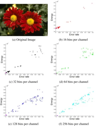
The GrabCut method can be seen as a block-coordinate descend and as such is prone to local

minimum. This problem is especially prominent when the number of parameters used to model

appearance is high, which is confirmed empirically in our experiments (see Fig. 3.1). We

randomly select box as initial solution. Region inside the box is taken as foreground and outside

as background. We run block-coordinate descent until convergence and do this experiment for

500 randomly generated boxes. For the 500 solutions we get, we compute their error rates and

energy. As we can see from the scatter plots, when the number of color bins increases, there

are more distinct solutions. This implies there are more local minima with more color bins and

GrabCut is more prone to getting stuck in local minima.

(a) Original Image (b) 16 bins per channel

(c) 32 bins per channel (d) 64 bins per channel

(e) 128 bins per channel (f) 256 bins per channel

3.2

Branch-and-Mincut

Branch-and-Mincut [40] combines two powerful techniques: Graph cut and Branch-and-Bound.

It can find global optimal of the energy (1.13), rather than local minima when using EM-style

GrabCut (Fig. 3.2). Branch-and-Bound is a popular optimization technique for combinatorial

optimization and discrete optimization. The basic idea of Branch-and-Bound is to divide the

space of all solutions into subsets and obtain a lower bound for each subset. Whenever the

lower bound of some subset is greater than the function value of current best solution, we can

prune those subsets and the search space is reduced. The search space is split, bounded and

pruned until only one solution is left, guaranteed to be the global optimum.

Figure 3.2: Branch-and-Mincut [40] can find smaller global energy while GrabCut gets stuck in local minima with larger energy.

For image segmentation with Graph cut, the search space is divided into subsets based on the

parameters of the appearance models. The lower bound of the appearance model subset can be

computed using a single run of maxflow algorithm.

If we use K bin color histogram as appearance model, the size of the search space for fore-ground and backfore-ground appearance models would be 22K_{. The time complexity of}

Branch-and-Mincut is exponential with respect to the number of color bins K. While finer color his-tograms can better describe appearance models, Branch-and-MinCut method cannot be used

due to exponential complexity.

Note that Branch-and-Mincut is not limited to optimization acceleration for choosing better

appearance model. It can also be applied to a wider range of graph cut problems as long as the

graphs are parameterized and have similar structure. For example, the shape matching problem

3.3

Dual Decomposition

Vincente et al. [59] proposed dual decomposition method to optimize the energy (1.13). First,

the energy is rewritten as:

E(S) = −

∑

i

h_Ωi(Si)+|∂S|−<y,S > +hΩ(S)+<y,S > (3.2)

wherey ∈ RN is a vector, N = |Ω|and < ·,· > is the dot product between two vectors. The followingΦ(y) gives a lower bound ofE(S):

Φ(y) = min

S [−

∑

i

h_Ωi(Si)+|∂S|−< y,S >]+min

S [hΩ(S)+< y,S >]. (3.3)

It suffices to considery= λ·1whereλis a scalar and1is a unit vector. So we can also rewrite the original energy as

E(S) = −∑

i

h_Ωi(Si)+|∂S| −λ <1,S >+hΩ(S)+λ <1,S > . (3.4)

We denote−∑_ih_Ωi(Si)+|∂S| −λ <1,S >asE1(S, λ) andhΩ(S)+λ <1,S >asE2(S, λ), then

we have

ϕ(λ)=argmin

S E

1_{(S, λ)+argmin}

S E

2_{(S, λ)≤E(S). (3.5)}

ϕ(λ) renders a lower bound of E(S) and is called the dual function of E(S). We can explore all values ofλto get the tightest lower bound. In order to optimize overλ, Vicente et al. [59] proposed using parametric maxflow, which is very slow in practice. If there is no discrepancy

between the lower bound at the optimalλand the original energy for the correspondingS, we obtain a global optimal solution. The final labeling is chosen among all solutions according

to the original energy. Dual decomposition is very slow in practice because to explore all

breakpoints via parametric-maxflow is slow.

3.4

Active Contour

Michailovich et al. in [45] proposed an active contour method that maximizes the

Bhat-tacharyya distance between foreground and background color distributions. The energy

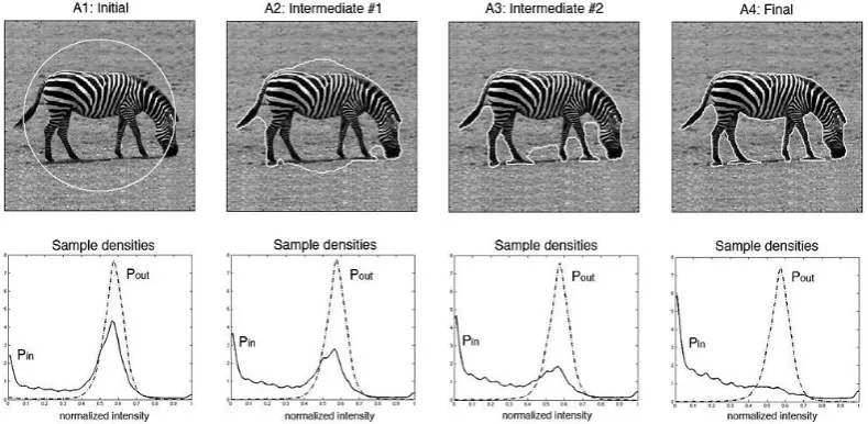
Figure 3.3: (top row) Intensity-based segmentation of Zebra at each iteration. (bottom row) Corresponding intensity distributions of Zebra and its background. Pinand Poutare intensity distributions of regions inside and outside the contour. [45]

evolution of the active contours at each iteration. Fig. 3.3 illustrates intermediate active

con-tours at different iterations and the corresponding foreground and background distributions.

As we can see, the final segmentation yields large discrepancy between foreground and

back-ground appearance distributions. The level set based method does not guarantee global optimal

Minimizing Appearance Overlap in

One-cut

In this chaper we introduce the L1 color separation term and show how it can be optimized

in one graph cut. We also talk about general color separation term that is not based on L1

metric. Particularly, we address the difference between our color separation term and Pn_potts

model which was originally proposed for enforcing labeling consistency within superpixels.

Note that the color separation terms here are all used for color histogram appearance model.

In this chapter, color separation terms are formulated over color histograms.Chapter 6shows

possible extensions to GMM appearance models.

4.1

L

Color Separation Term

Let S ⊂ Ω be a segment of the image plane Ω and denote by θS _{and θ}S¯ _{the unnormalized}

color histograms for the foreground and background appearance respectively. Let nk be the

number of pixels in the image that belong to bink and letnS_k andnS_k¯ be the according number of the foreground and background pixels in bink. Our appearance overlap term penalizes the intersection between the foreground and background bin counts by incorporating the simple

yet effective high-orderL1 term into the energy function:

EL1(θ

S_{, θ}S¯_)=−∥θS _−θS¯_∥

L1, (4.1)

Theorem 4.1.1. The L1color separation term we proposed here is submodular.

Below we explain how to incorporate and optimize the term EL1(θ

S_{, θ}S¯_{) using one graph}

Figure 4.1: Graph construction forEL1 in one color bin: nodesv1,v2, . . . ,vnk corresponding to

the pixels in binkare connected to the auxiliary nodeAk using undirected links. The capacity

of these links is the weight of appearance overlap termβ >0.

cut. For clarity of explanation we rewrite the term as

EL1(θ

S_{, θ}S¯₎₌ K

∑

k=1

min(nS_k,nS_k¯)− |Ω|

2 . (4.2)

It is easy to show that the two sides of (4.2) are equivalent. It’s obvious that the L1 color

separation term encourages labeling inconsistency among pixels in the same color bin. The

details of the graph construction for the above term over one color bin are shown in Fig. 4.1.

In the graph we ignore links for other terms such as smoothness term.

Figure 4.2: Overall graph construction for energy withL1color separation term. We have three

Fig. 4.2 gives the overall graph construction of energy withL1color separation term. We add

K auxiliary nodesA1,A2, ...,AK into the graph and connectkthauxiliary node to all the pixels

that belong to the kth bin. In this way each pixel is connected to its corresponding auxiliary node. The capacity of these links is set toβ= 1. Assume that binkis split into foreground and background, resulting innS

k andn

¯

S

k pixels accordingly. Then any cut separating the foreground

and background pixels must either cut nS k or n

¯

S

k links that connect the pixels in bin k to the

auxiliary nodeAk. The optimal cut must choose min(nS_k,n

¯

S

k) in (4.2).

4.2

Minimizing Higher-order Pseudo-boolean Function

TheL1color separation term can be seen as a special case of the following higher-order

psudo-boolean function:

f(Xc)= min{θ0+ ∑

i∈c

w0_i(1−xi), θ1+ ∑

i∈c

w1_ixi, θmax} (4.3)

where xi ∈ {0,1} are binary variables in clique c, w0_i > 0, w1_i > 0, and θ0, θ1 and θmax are

parameters satisfying the constraints θmax > θ0 and θmax > θ1. Consider each color bin as a

clique and set parametersw0_i = 1, w1_i = 1, θ0 = 0, θ1 = 0 andθmax = nk/2, where nk is the

number of pixels in bink. Then f(Xc) reduces toEL1(θ

S_{, θ}S¯_)+|Ω|/2.

Figure 4.3: Our graph for minimizing pseudo-boolean function (4.3), r = min{θ0, θ1}. Note

We also propose graph construction (Fig. 4.3) for minimizing pseudo-boolean functions in

(4.3) using directed links. Note how the graph in Fig. 4.3 degenerates to the graph in Fig. 4.1:

If θmax = +∞ andθ0 = θ1 = 0, then the two nodes A1_k and A0_k emerge to one node, directed

link becomes undirected and the auxiliary nodes are disconnected from source or sink nodes

becauseθ1−r =0 andθ0−r= 0.

To see how the graph in Fig. 4.3 works we consider four possible label assignments for the

auxiliary nodes A1

k andA

0

k. Table 4.1 shows the cost of corresponding cuts. The minimum cut

renders optimization of the function (4.3).

(A1_k,A0_k) the cost of cut (0,0) θ1+

∑

i|xi=1w

1

i −r

(0,1) θ0+ ∑

i|xi=0w

0

i +θ1+

∑

i|xi=1w

1

i −2r

(1,0) θmax−r

(1,1) θ0+ ∑

i|xi=0w

0

i −r

Table 4.1: Cut costs corresponding to four possible label assignments to the binary auxiliary n-odesA1

k andA

0

k. The optimal cut must choose the minimum of the above costs, thus minimizing

(4.3).

4.3

Relationship with

P

Potts Model

A similar graph construction with auxiliary nodes (Fig. 4.4) is proposed in [30, 31] to minimize

higher order pseudo-boolean functions (4.3).

Unlike our construction, the method in [30, 31] requires that the parameterθmaxin f(Xc) should

satisfy the following constraint:

θmax 6max(θ0+ ∑

i∈c

w0_i(1−xi), θ1+ ∑

i∈c

w1_ixi). (4.4)

In contrast, we can optimize high-order functions in (4.3) with arbitrary θmax provided that

θmax > θ0 and θmax > θ1. Even though the constraint is not problematic for color separation

term as long as we setθmax tonk/2, but we believe eliminating the constrain is important for

some other applications when the constraint cannot be easily satisfied.

The graph construction in Fig. 4.4 can be used to minimize EL1. However, the advantage of our graph construction in Fig. 4.1 is that only one auxiliary node is needed for each color bin,

Figure 4.4: Graph for minimizing pseudo-boolean function (4.3) by Kohli et al. [30, 31]

4.4

General Color Separation Term

In general, color separation term does not have to be based onL1distance. We can define color

separation term using other distance metric such as Jensen-Shannon distance, χ2 _{distance or}

Bhattacharyyadistance. For example, below we define four appearance overlap terms based on the L1 norm, χ2 distance, Bhattacharyya coefficient and Jensen-Shannon divergence between

histograms.

DL1(θ

S_{, θ}S¯₎₌ K

∑

k=1

min (nS_k,nS_k¯) (4.5)

D_χ2(θS, θS¯)=

K

∑

k=1

(nk/2−(nSk −n

¯

S k)

2_/(2n

k)) (4.6)

DBha(θS, θ

¯

S₎₌ K

∑

k=1 √ nS kn ¯ S k (4.7)

DJS(θS, θ

¯

S

)=

K

∑

k=1

nklognk−nS_k lognS_k −nS_k¯lognS_k¯

2 (4.8)

Figure 4.5: Appearance overlap terms based on different metrics: L1norm,χ2 distance,

Bhat-tacharyya coefficient and Jensen-Shannon divergence

All four terms above are concave functions ofns

k attaining maximum atnk/2. See Fig. 4.5 for

the visualization of the terms and comparison withDL1.

Similarly to [30] we observe that any concave function can be approximated as a piece-wise

lin-ear function by using a summation of specific (pyramid-like) truncated functions, each having

a general form as in (4.3). For example, Fig. 4.6 illustrates one possible approximation using

three components. These truncated components take the form of high-order psudo-boolean

function in (4.3) and thus can be incorporated into our graph using the construction shown in

Fig. 4.3. Note, DL1 is equivalent toDχ2, DBha orDJS when approximated using one truncated component.

Applications

In this section we apply our appearance overlap penalty term in a number of different

practi-cal applications including interactive binary segmentation with bounding boxes or strokes in

Sec.5.1, shape matching with simple shape templates in Sec.5.2, saliency segmentation with

saliency maps in Sec.5.3 and segmentation from stereo pairs in Sec. 5.4. We show general

usefulness of our proposed color separation term.

5.1

Interactive segmentation

First, we discuss interactive segmentation with several standard user interfaces: bounding box

[51] in Section 5.1.1 and seeds [12] in Section 5.1.3. We compare different color separation

terms includingL1, Jenson-Shannon, Bhattacharyya,χ2and truncatedL1color separation terms

in Section 5.1.2.

5.1.1

Binary segmentation with bounding box

First, we use appearance overlap penalty in a binary segmentation experiment with the same

setting as GrabCut [9, 51]. For GrabCut GMM is used as appearance model but here color

histogram is the appearance model. A user provides a bounding box around an object of interest

and the goal is to perform binary image segmentation within the box. The pixels outside the

bounding box are assigned to the background using hard constraints. The hard constrain is

achieved by having infinity edge weights for links connecting these pixels and sink node. Let

R ⊆ Ω denote the binary mask corresponding to the bounding box, SGT ⊆ Ω be the ground

truth foreground and S ⊆ Ω be a segment. Denote by 1S = {sp|p ∈ Ω} the characteristic