CHALLENGES FACED DURING THE MODELLING, DYNAMIC
ANALYSIS, AND VULNERABILITY STUDY WITH SOFISTIK IN THE
CONTEXT OF THE SMART 2013 BENCHMARK PROJECT
Rainer Zinn1, Michael Borgerhoff 1, Claudia van Exel1, Urs Bumann2, and Tadeusz Szczesiak2
1
Stangenberg und Partner Consulting Engineers, Germany ([email protected])
2
Swiss Federal Nuclear Safety Inspectorate ENSI, Switzerland
ABSTRACT
The international benchmark project SMART 2013 that has been supported by CEA and EDF under the hospice of the IAEA aims at understanding the nonlinear response of a typical nuclear reinforced concrete (RC) structure subjected to high intensity seismic loading. An experimental campaign on a new mock-up, which has been launched in 2013 and has been carried out at Centre de Saclay/EMSI, provided reference data for the project. This paper describes the work conducted by the “ENSI Team 2”, consisting of the Swiss Federal Nuclear Safety Inspectorate (ENSI) and the Stangenberg & Partner Consulting Engineers (SPI), in the context of the benchmark project. The paper focuses on the challenges faced during the modelling procedure, on the findings gained from the comparison between the accelerations and displacements predicted by the numerical model and the measured experimental results, and the vulnerability study with establishing of different fragility curves.
INTRODUCTION
As part of “SMART 2008 project”, a reduced scale model (1/4th scale) representative of a typical, simplified half part of an electrical nuclear building was designed, built and tested in 2008 on the AZALEE shaking table from TAMARIS experimental platform from EMSI laboratory in SEMT service in order to access the capability of buildings to withstand earthquake loading as well as seismic loads induced to their equipment, see Lermitte et al. (2009). To improve the knowledge of the seismic behaviour of such RC structures, a new research program was started in 2011, namely “SMART 2013 project”, see Richard et al. (2014).
The test mock-up of SMART 2013 project is shown in Figure 1. The dimensions of the mock-up are 3.6m height and 3.1m x 2.55m in plan. The overall mass is 45.8t including the additional loads on the floors, and 70.8t including the AZALEE shaking table.
Figure1. SMART 2013 project: test mock-up
DEVELOPMENT OF THE NUMERICAL MODEL
The verification analyses have been performed with a Finite Element (FE) model of the mock-up by use of the computer program SOFiSTiK, see SOFiSTiK AG (2010). The concrete floor slabs, the walls, and the column are modelled by shell elements. The analysis of nonlinear effects in SOFiSTiK is done by iterations using a modified Newton method; i.e. an implicit integration scheme is used. The calculation code SOFiSTiK is well-suited for linear and nonlinear analysis of RC targets subjected to seismic or impact loads, see Borgerhoff et al. (2013), Moore et al. (2013). In the SOFiSTiK code, the RC structure is modelled with nonlinear, layered shell elements; nonlinear shear deformations of shell/plate elements are approximately included. A partition into 12 layers is sufficient according to our experience and is used in the performed analyses. The nonlinear material behaviour of reinforced concrete in the shell elements is regarded by use of a layer model with correct positioning of the crosswise arranged layers of bending reinforcement in the represented section. The nonlinear behaviour of the components of reinforced concrete is defined by
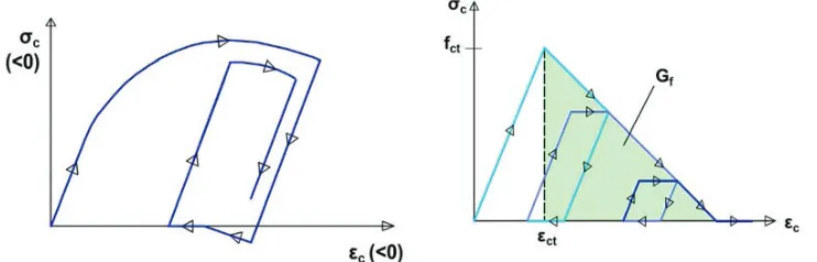
• nonlinear uniaxial stress-strain relationship for concrete including hysteretic behaviour as shown for
concrete in compression in Figure 2 (including increase in strength due to biaxial compressive behaviour),
• consideration of tension softening of concrete after cracking dependent on fracture energy with
hysteretic behaviour as shown in Figure 2,
• approximate inclusion of transverse shear deformations by an elastic/ideally plastic shear stress/shear strain law after exceeding the specified ultimate shear strength, and
• trilinear stress-strain relationship for reinforcing steel with hysteretic behaviour.
Figure 2. Hysteretic envelopes of concrete in compression (left) and in tension (right) (SOFiSTiK approach).
The different FE models are depicted in Figure 3. The model with shaking table, which was used for stages #2 and #3, comprises 9,942 shell elements and 49,600 DOF, where the shaking table AZALEE was adopted from the SAP2000 model as submitted by CEA. The model with support springs, which was used for stage #4, comprises 4,085 shell elements and 26,900 DOF. The model masses are: mock-up 47.0t (CEA 45.8t), mock-up linked to shaking table 70.6t (CEA 70.8t).
Figure 3. SOFiSTiK FE models including shaking table (left, stages #2, 3) and with support springs (right, stage #4)
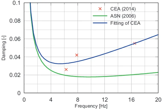
Damping is introduced by means of Rayleigh damping parameters Į and ȕ which are introduced in two
Figure 4. Damping values introduced by Rayleigh parameters vs values given by CEA Richard et al. (2014)
ELASTIC CALIBRATION OF THE NUMERICAL MODEL
The elastic calibration (stage #2) comprises modal analysis with different boundary conditions (mock-up fixed and linked to the shaking table model), and transient analyses Run 6 and Run 7. Table 1 summarizes the first three frequencies for different boundary conditions in comparison with the data Richard et al. (2014). “AZALEE” in Table 1 means that the AZALEE shaking table is treated alone (without mock-up). “Fixed” means that the mock-up with fixed base is treated alone, and “Linked to shaking table” means that the coupled system mock-up / AZALEE shaking table is treated.
Table 1. Comparison of frequencies for different boundary conditions
Frequency SOFiSTiK
AZALEE with air cushions
SOFiSTiK Fixed, add. masses
SOFiSTiK Linked to shaking table
CEA AZALEE with air cushions
CEA Fixed, add. masses
CEA Linked to shaking table
1st 81.3Hz 8.2Hz 5.84Hz 80.5Hz 8.98Hz 6.28Hz
2ŶĚ
96.2Hz 15.1Hz 9.09Hz 95.7Hz 15.54Hz 7.86Hz
3ƌĚ
118.0Hz 28.4Hz 19.50Hz 116.2Hz 31.50Hz 16.50Hz
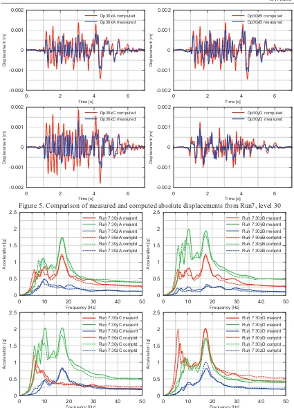
Run 6 and Run 7 were performed with the damping parameters fitted to the CEA damping values. The seismic excitation was applied in terms of absolute displacements of the AZALEE accelerators. Since there were problems with respect to the provided data for Run 6 (e.g., the second derivatives of the absolute displacements substantially differ from the absolute accelerations due to filtering effects), in the following only results from Run 7 are documented. Figures 5 and 6 show a comparison of measured and computed values of selected absolute displacements and acceleration response spectra for Run 7. The computed displacements and low frequency spectral accelerations are slightly higher than the measured values, likely due to real modal damping values higher than the values introduced in the computation.
0 4 8 12 16 20
Frequency [Hz] 0
0.02 0.04 0.06 0.08 0.1
D
a
m
p
in
g
[-]
Figure 5. Comparison of measured and computed absolute displacements from Run7, level 30
Figure 6. Comparison of acceleration response spectra from Run 7, level 30, damping 5%
0 2 4 6
Time [s] -0.002 -0.001 0 0.001 D is p la c e m e n t [m ] Dp30xA computed Dp30xA measured
0 2 4 6
Time [s] -0.002 -0.001 0 0.001 D is p la c e m e n t [m ] Dp30xB computed Dp30xB measured
0 2 4 6
Time [s] -0.002 -0.001 0 0.001 0.002 D is p la c e m e n t [m ] Dp30xC computed Dp30xC measured
0 2 4 6
Time [s] -0.002 -0.001 0 0.001 0.002 D is p la c e m e n t [m ] Dp30yD computed Dp30yD measured
0 10 20 30 40 50
Frequency [Hz] 0 0.5 1 1.5 2 2.5 A c c e le ra ti o n [g ]
Run 7 30xA measrd Run 7 30yA measrd Run 7 30zA measrd Run 7 30xA comptd Run 7 30yA comptd Run 7 30zA comptd
0 10 20 30 40 50
Frequency [Hz] 0 0.5 1 1.5 2 2.5 A c c e le ra ti o n [g ]
Run 7 30xB measrd Run 7 30yB measrd Run 7 30zB measrd Run 7 30xB comptd Run 7 30yB comptd Run 7 30zB comptd
0 10 20 30 40 50
Frequency [Hz] 0 0.5 1 1.5 2 2.5 A c c e le ra ti o n [g ]
Run 7 30xC measrd Run 7 30yC measrd Run 7 30zC measrd Run 7 30xC comptd Run 7 30yC comptd Run 7 30zC comptd
0 10 20 30 40 50
Frequency [Hz] 0 0.5 1 1.5 2 2.5 A c c e le ra ti o n [g ]
NONLINEAR DYNAMIC BEHAVIOUR OF THE NUMERICAL MODEL AND COMPARISON WITH TEST RESULTS
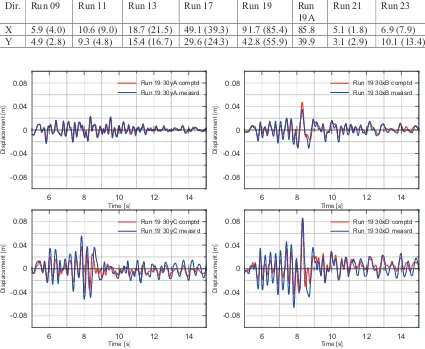
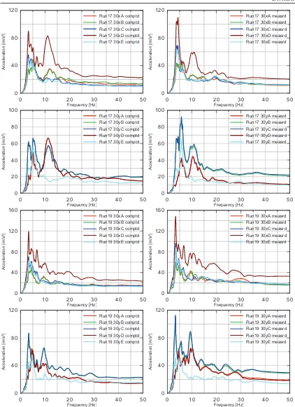
The nonlinear dynamic analysis (stage #3) comprises nonlinear step-by-step integration computations of the coupled system consisting of mock-up linked to the shaking table model. All runs – mandatory runs as well as optional runs – were performed in a sequential series, i.e. considering the pre-damage of the respective preceding run. The seismic excitation was applied in terms of absolute displacements of the AZALEE accelerators with a time step of 0.003908s. The damping parameters were introduced according to the French seismic guide ASN (2006). For Run19 – excitation Northridge earthquake (1994) with the largest PGA values up to 1.1g (design value of mock-up: 0.2g) – the damping values fitting the CEA data have been used alternatively. From the numerous results, only a small selection can be presented in this paper. In Table 2 the maximum computed absolute displacements are tabulated in comparison with the measured data. The displacements are corrected with respect to the initial displacements due to residual displacements of the respective preceding run. Figures 7 and 8 show selected displacements and acceleration response spectra.
Table 2. Comparison of maximum absolute displacements in mm, values in ( ) are measured displacements (Run19A = Run19 with CEA damping values)
Dir. Run 09 Run 11 Run 13 Run 17 Run 19 Run
19A
Run 21 Run 23
X 5.9 (4.0) 10.6 (9.0) 18.7 (21.5) 49.1 (39.3) 91.7 (85.4) 85.8 5.1 (1.8) 6.9 (7.9)
Y 4.9 (2.8) 9.3 (4.8) 15.4 (16.7) 29.6 (24.3) 42.8 (55.9) 39.9 3.1 (2.9) 10.1 (13.4)
Figure 7. Comparison of selected computed and measured absolute displacements
6 8 10 12 14
Time [s]
-0.08 -0.04 0 0.04 0.08
D
is
p
la
c
e
m
e
n
t
[m
]
Run 19 30yA comptd Run 19 30yA measrd
6 8 10 12 14
Time [s]
-0.08 -0.04 0 0.04 0.08
D
is
p
la
c
e
m
e
n
t
[m
]
Run 19 30xB comptd Run 19 30xB measrd
6 8 10 12 14
Time [s]
-0.08 -0.04 0 0.04 0.08
D
is
p
la
c
e
m
e
n
t
[m
]
Run 19 30yC comptd Run 19 30yC measrd
6 8 10 12 14
Time [s]
-0.08 -0.04 0 0.04 0.08
D
is
p
la
c
e
m
e
n
t
[m
]
Figure 8. Comparison of acceleration response spectra, level 30, damping 5%
0 10 20 30 40 50
Frequency [Hz] 0 40 80 A c c e le ra ti o n [m /s ²]
Run17 30xA comptd Run17 30xB comptd Run17 30xC comptd Run17 30xD comptd Run17 30xE comptd
0 10 20 30 40 50
Frequency [Hz] 0 40 80 A c c e le ra ti o n [m /s ²]
Run17 30xA measrd Run17 30xB measrd Run17 30xC measrd Run17 30xD measrd Run17 30xE measrd
0 10 20 30 40 50
Frequency [Hz] 0 20 40 60 80 100 A c c e le ra ti o n [m /s ²]
Run17 30yA comptd Run17 30yB comptd Run17 30yC comptd Run17 30yD comptd Run17 30yE comptd
0 10 20 30 40 50
Frequency [Hz] 0 20 40 60 80 100 A c c e le ra ti o n [m /s ²]
Run17 30yA measrd Run17 30yB measrd Run17 30yC measrd Run17 30yD measrd Run17 30yE measrd
0 10 20 30 40 50
Frequency [Hz] 0 40 80 120 160 A c c e le ra ti o n [m /s ²]
Run19 30xA comptd Run19 30xB comptd Run19 30xC comptd Run19 30xD comptd Run19 30xE comptd
0 10 20 30 40 50
Frequency [Hz] 0 40 80 120 160 A c c e le ra ti o n [m /s ²]
Run19 30xA measrd Run19 30xB measrd Run19 30xC measrd Run19 30xD measrd Run19 30xE measrd
0 10 20 30 40 50
Frequency [Hz] 0 40 80 120 A c c e le ra ti o n [m /s ²]
Run19 30yA comptd Run19 30yB comptd Run19 30yC comptd Run19 30yD comptd Run19 30yE comptd
0 10 20 30 40 50
Frequency [Hz] 0 40 80 120 A c c e le ra ti o n [m /s ²]
VULNERABILITY STUDY AND REMARKS ON THE FRAGILITY CURVES
The vulnerability study (stage #4) is focused on the probabilistic evaluation of the mock-up vulnerability. The determination of fragility curves with respect to prescribed criteria is the main objective of this stage. For the vulnerability analysis, the FE model of the mock-up resting on support springs was used, see Fig. 3. The random variables for concrete tensile strength, concrete structural damping ratio, spring stiffness and dampers were adopted from ENSI team 1, see Sevdali et al. (2014). The mandatory 50 sets of horizontal accelerogram pairs as provided by CEA were used (49 accelerogram pairs are included in the fragility curve evaluation, because for Run 35 the structure failed). A simplified method for
determining the fragility curves based on a linear regression in order to evaluate the two parameters Am
and ȕ was used. The seismic demand model is described with
İ + ) ( b + a =
(Y) ln Θ
ln (1)
where İ is a centered normal (Gaussian) random variable with standard deviation ı, and a, b are constants
that are evaluated by means of linear regression. Ĭ is the treated ground motion parameter (PGA, ASA40,
CAV), and Y is the model output (drift, frequency drop). With these notations, the corresponding lognormal fragility curve is
¸¸ ¹ · ¨¨
©
§ Θ
Θ
σ /s) (a )=ĭ ( P
b
f
ln
(2)
where s is the threshold of the ground motion parameter Y. The fragility curve, that is the failure
probability Pf conditioned on ground motion parameter Ĭ, is given by the cumulative distribution function
¸¸ ¹ · ¨¨
©
§ Θ
= Θ
ȕ ) /A ( ĭ ) (
P m
f
ln
(3)
where Am = exp((ln(s)-a)/b) is the median seismic capacity and ȕ = ı / b is the standard deviation of the
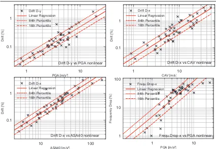
fragility curve. Figures 9 and 10 show examples of the performed regression analyses. There are good correlations for the output parameter storey drift, expressed by coefficients of determination of 0.8 - 0.9, but only poor correlations for the output parameter frequency drop, characterized by coefficients of determination of 0.6 - 0.7. Examples of resulting fragility curves are shown in Figures 11 and 12 for the case “extended damage”, i.e. thresholds storey drift h/100 and frequency drop 50%.
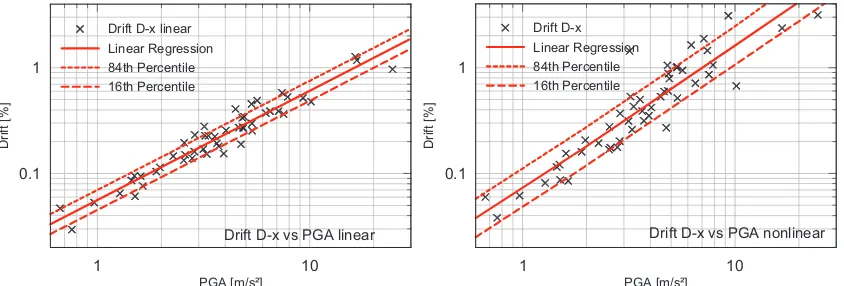
Figure 9. Regression analysis for ground motion parameter PGA-X and storey drifts D-x from linear (left) and nonlinear (right) computations
1 10
PGA [m/s²]
0.1 1
D
ri
ft
[%
]
Drift D-x linear Linear Regression 84th Percentile 16th Percentile
Drift D-x vs PGA linear
1 10
PGA [m/s²]
0.1 1
D
ri
ft
[%
]
Drift D-x Linear Regression 84th Percentile 16th Percentile
Figure 10. Regression analysis from nonlinear computations for selected ground motion and output parameters
Figure 11. Fragility curves for extended damage level (storey drift h/100, frequency drop 50%) for ground motion parameters PGA (left) and CAV (right)
1 10
PGA [m/s²]
0.1 1
D
ri
ft
[%
]
Drift D-y Linear Regression 84th Percentile 16th Percentile
Drift D-y vs PGA nonlinear
1 10
CAV [m/s]
0.1 1
D
ri
ft
[%
]
Drift D-x Linear Regression 84th Percentile 16th Percentile
Drift D-x vs CAV nonlinear
10 100
ASA40 [m/s³]
0.1 1
D
ri
ft
[%
]
Drift D-x Linear Regression 84th Percentile 16th Percentile
Drift D-x vs ASA40 nonlinear
1 10
PGA [m/s²]
1 10 100
F
re
q
u
e
n
c
y
D
ro
p
[%
]
Frequ.Drop-x Linear Regression 84th Percentile 16th Percentile
Frequ.Drop-x vs PGA nonlinear
1 10
PGA [m/s²]
0 20 40 60 80 100
F
a
ilu
re
P
ro
b
a
b
ili
ty
[%
]
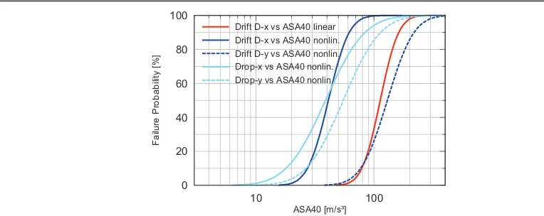
Drift D-x vs PGA linear Drift D-x vs PGA nonlin. Drift D-y vs PGA nonlin. Drop-x vs PGA nonlin. Drop-y vs PGA nonlin.
1 10 100
CAV [m/s]
0 20 40 60 80 100
F
a
ilu
re
P
ro
b
a
b
ili
ty
[%
]
Figure 12. Fragility curves for extended damage level (storey drift h/100, frequency drop 50%) for ground motion parameter ASA40
There are clear correlations between the ground motion parameters PGA, CAV, ASA40 and the response parameter storey drift. But, for the frequency drop as a response parameter, a clear correlation could not be observed. It should be mentioned that the frequency drops were estimated from the decrease of peaks of Fourier spectra of displacements, which likely is not a very stable procedure.
CONCLUSIONS
The linear and nonlinear dynamic seismic response analyses in the frame of the SMART 2013 project with the FE program SOFiStiK showed a good agreement between computed and measured values up to extreme earthquake loads of 1.1g (design value of mock-up: 0.2g). The use of the damping values according to the regulation in ASN (2006) for nonlinear seismic analysis yielded computed structural responses comparable to measured results. The vulnerability analysis yielded plausible correlations between the ground motion parameters PGA, CAV, ASA40 and the response parameter storey drift. But, for the response parameter frequency drop, no clear correlations could be observed.
REFERENCES
Borgerhoff, M., Schneeberger, C., Stangenberg, F., and Zinn, R. (2013). „Conclusions from Combined
Bending and Punching Tests for Aircraft Impact Design”, Transactions SMiRT-22, San Francisco,
USA.
Lermitte, S., Chaudat, T., Courtois, A. (2009). “SMART 2008 Project Experimental Tests of a Reinforced Concrete Building Subjected to Torsion, Part 2: Presentation of the Test Results”, Transactions SMiRT-20, Espoo, Finland.
Moore, J., Zwicky, P., Zinn, R., and Schneeberger C. (2013). „Earthquake Response Analysis in the
Context of the KARISMA Benchmark Project”, Transactions SMiRT-22, San Francisco, USA.
ASN (2006), ”Prise en compte du risque sismique à la conception des ouvrages de genie civil d’installations nucléaires de base à l’exception des stockages à long terme des déchets radioactifs”, ASN/Guide/2/01.
Richard, B., Charbonell, P. E. (2014). “Presentation of the SMART 2013 International Benchmark”,
Report DEN/DANS/SET/EMSI/ST/12-017/H, 09/04/2014.
Sevdali, I., Billmaier, M, Mondet, Y., Szczesiak, T. Bumann, U., (2014). “SMART2013, ENSI Team 1: Challenges faced during the modelling, dynamic analysis, and vulnerability study with SAP2000
using nonlinear layered shell elements”, Workshop SMART 2013, Paris, France.
SOFiSTiK AG (2010), „SOFiSTiK, Analysis Programs“, Version 25.0, Oberschleissheim.
10 100
ASA40 [m/s³]
0 20 40 60 80 100
F
a
ilu
re
P
ro
b
a
b
ili
ty
[%
]