Sin-Cos-Taylor-Like method for solving stiff ordinary
diffrential equations
Rokiah @ Rozita Ahmad*, Nazeeruddin Yaacob
Mathematics Department, Faculty Of Sciences, Universiti Teknologi Malaysia, 81310 UTM Skudai, Johor, Malaysia *To whom correspondence should be addressed. E-mail: [email protected]
Received 8 November 2005
ABSTRACT
This paper discusses the derivation of an explicit Sin-Cos-Taylor-Like method for solving stiff ordinary differential equations, which is a formulation of the combination of a polynomial and the exponential function. This new method requires extra work to evaluate a number of differentiations of the function involved. However, the result shows smaller errors when compared to the results from the explicit classical fourth-order Runge-Kutta (RK4) and the Adam-Bashforth-Moulton (ABM) methods. Implicit methods could work well for stiff problems but have certain drawbacks especially when discussing about the cost. Although extra work is required, this explicit method has its own advantages. Besides providing excellent results, the cost of computation using this explicit method is much cheaper than the implicit methods. We also considered the stability property for this method since the stability property of the classical explicit fourth order Runge-Kutta method is not adequate for the solution of stiff problems. As a result, we find that this explicit method is of order-6, which has been developed, and proved to be both A-stable and L-stable.
| Stiff ordinary differential equations | Explicit methods |A-stable |L-stable |
1. Introduction
Stiff problem entails rapidly decaying transient solution, which arises naturally in wide variety of applications including the study of spring and damping system, the analysis of control system and problems in the chemical kinetics [1]. Stiff differential equations also occur in other kind of studies, such as biochemistry, biomedical system, weather prediction, mathematical biology and electronics. In chemical kinetics, stiffness is caused in the vast majority of cases merely by a great difference among the reaction rate constants. This problem is more likely to occur whenever we have a larger system or the more detail and complicated the models are. The atmospheric phenomena as an example, involves transport with chemical reaction, thus stiffness can occur because of the time scales of the reactions are much smaller than times for movement over distances. Stiffness in heat transfer originates physically in one of two ways; sharp changes in the thermal environment of large differences in the rates which components of the system can transfer heat [2].
Stiffness is generally understood in terms of what goes wrong when numerical methods not design for such problems are used to try to solve them [3]. Lambert in [4] points out that one should consider stiffness as a phenomenon exhibited by a system, rather than a property of it, because the word property is associated to the
Article
J
ournal of
F
undamental
S
ciences
Available online at
existence of a definition, which is both comprehensive and precise, whereas it is difficult to come out with a satisfactory definition for the concept of “stiffness”.
This paper focuses on the explicit one-step methods for solving stiff differential equations. Although most of the numerical analysts were confident that the implicit methods work better in producing results for stiff problems but this research meant to explore the explicit methods, which recently was proven, could also satisfy the stiff problems [5].
2. Formulation
Rokiah & Nazeeruddin [6] have shown that the explicit one-step method for stiff problems could be represented by the composition of a polynomial and exponential function of the form
2
0 1 2 3 4 5 1
( ) + (
( + (
(
))))
b tPE t
=
a t a
+
t a t a
+
t a
+
a t
+
Ab e
(1.1).
Taking A = 1, we calculated the values of ai , i = 0,1,2,3,4,5 and bi, i = 1,2. In [7], we substituted the constant A
=1 with a trigonometric function, sin znh. Based on the same theory for the solution of a differential equation
with complex eigenvalues, we replaced the constant A by sin znh + cos znh which produced a
Sin-Cos-Taylor-Like method. For simplicity we name this method as SCTL6 method. Provided that f (5). f (6)≠ 0, we obtained the equation
(4)
(5)
( ) 2 3
6
4
( )
(
)
(
)
(
)
(
)
(
)
2
6
24
120
(sin(
) cos(
))
1
1
1
(
)
( (
))
( (
))
2
6
1
1
( (
))
( (
24
120
n n n nn n n n n n n
z t t
n n n
n n n n n n
n
n n n
f
f
f
f
PE t
y
t t
f
t t
t t
t t
t t
f
z h
z h
e
z t t
z t t
z t t
z
z t t
z t
−
′
′′
′′′
=
+ −
+ −
+ −
+ −
+ −
+
+
− −
−
−
−
−
−
−
−
−
−
))
5n
t
(1.2)
where (6) (5) n n n
f
z
f
=
Letting t = tn+1, we arrive at the formula below:
(4) (5)
1 6
(sin(
) cos(
))
2
6
24
120
1
1
1
exp(
) 1
1
.
2
6
24 120
n n n n n n n
n n n
n
n
n n n n n
f
f
f
f
f
z h
z h
y
y
h f
h
h
h
h
z
z h
z h
hz
hz
hz
hz
+
′
′′
′′′
+
=
+
+
+
+
+
+
− −
+
+
+
+
3. Local Truncation Error
The local truncation error for this particular method given by the formula (1.3) can be represented by
1 1 1
2 3 4 5 6
(4) (5) (6)
(4) (5) 7 (6) 6
(
)
( )
( )
( )
( )
( )
( )
( )
2
6
24
120
720
( )
2
6
24
120
(sin(
) cos(
))
n n n
n n n n n n n
n n n n
n n
n n n
n
T
y t
y
h
h
h
h
h
y t
hy t
y t
y t
y
t
y
t
y
t
y
y
y
y
O h
y
h y
h
h
h
h
y
z h
z h
e
z
+=
+−
+′
′′
′′′
=
+
+
+
+
+
+
+
′′
′′′
′
−
−
+
+
+
+
−
+
1
1
1
1
1
2
6
24 120
n
z h n
n n n n
z h
z h
z h
z h
z h
− −
+
+
+
+
6
(6)
(1 (sin(
) cos(
)))
( ).
7720
n n nh
y
z h
z h
O h
=
−
+
+
With
6
(6) 7
1
720
(1 (sin(
) cos(
)))
( )
n n n n
h
T
+=
y
−
z h
+
z h
+
O h
, we conclude that the SCT-L6 method is a sixth-order method.
4. Stability
4.1. Theorem 1.1
The explicit Sin-Cos-Taylor-Like method is A-stable. Proof:
Applying equation (0.3) to the test equation, with Re (λ)< 0, we obtain
2 3 4 5
1
2
6
24
120
1
1
1
(sin(
) cos(
)) e
1
1
2
6
24 120
n n n n
n n n
h
n n
y
y
y
y
y
y
h
y
h
h
h
h
h
y
z h
h
λh
h
h
h
( ) ( )
( ) ( ) ( )
4 5
2 3
2 3 4 5
(
)
(
)
1
2
6
24
120
(
)
(sin(
) cos(
)) e
1
2
6
24
120
n h n n
h
h
h
h
y
h
h
h
h
h
y
z h
h
λh
λ
λ
λ
λ
λ
λ
λ
λ
λ
λ
λ
=
+
+
+
+
+
+
+
− +
+
+
+
+
(
2 3 4 5
e (sin(
) cos(
) (1 (sin(
) cos(
)))
(
)
(
)
(
)
(
)
1
2
3!
4!
5!
h n
y
h
h
h
h
h
h
h
h
h
λλ
λ
λ
λ
λ
λ
λ
λ
λ
=
+
+ −
+
+
+
+
+
+
which leads us to yn+1= G (λh) yn;
(
)
e [sin(
h) cos(
)] [1 (sin(
) cos(
))]
h hG h
h
h
h
h e
e
λ λ
λ
λ
≈
λ
+
λ
+ −
λ
+
λ
=
Sinceyn+1
≈
eλh yny1
≈
eλh y0 ; y2≈
eλh y1≈
e 2λh y0 … yk≈
eλh yk –1≈
e kλh y0For any fixed pointt = tn = nh, we have
yn
≈
e
n hλ y0.Since|enλh|→ 0 as n→∞for all λh with Re (λ)< 0, we have yn→ 0 as n→∞ and consequently the method is A
-stable.
4.2. Theorem 1.2
The explicit Sin-Cos-Taylor-Like method is also L-stable. Proof:
Applying equation (0.3) to the test equation, with Re (λ)< 0, we obtain yn+1 ≈ eλhyn
From Theorem 1.1, the method is A-stable.
Since |eλh|→ 0 as Re(λh)→−∞, we have L-stability.
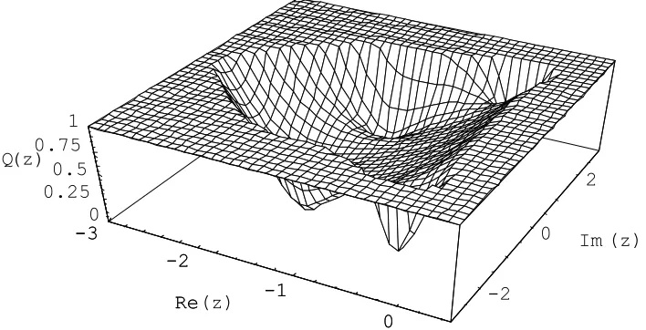
Fig. 1 The stability region of the SCTL6 method in 3D.
-3 -2.5 -2 -1.5 -1 -0.5 0 0.5
-3 -2 -1 0 1 2 3
Fig. 2 The stability region in 2D given by the SCTL6 method.
-1
0
Re -2
Q
-1
0 Re
-3
-2
(z)
0 2
Im(z)
0 0.250.5 0.75
1 (z)
-3
5. Numerical Results and Discussion
The formula [1.4] is tested on the stiff ordinary differential equation
'( )
100 ( ) 99
ty t
= −
y t
+
e
− ,y
(0) =0,
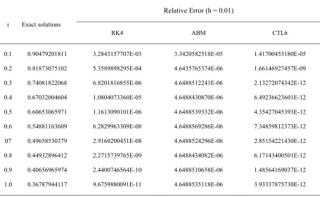
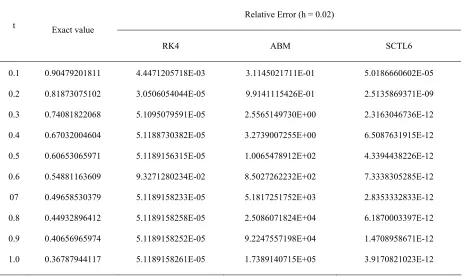
(3.1)and compared to the exact solution using the step size, h = 0.01 and h = 0.02 . We also solve equation (3.1) using another two established methods, namely the classical fourth-order Runge-Kutta (RK4), the implicit Adam-Bashforth-Moulton (ABM) methods. The relative errors for the methods applied, with the two different step sizes are compared and presented in Table 1 and 2. Table 3 shows the number of function evaluation in each iteration for the RK4, ABM and SCTL6 methods.
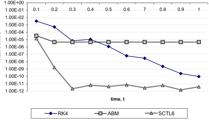
Figure 3 and 4 exhibits the graphs of the relative errors for all the methods used while in Figure 5 and 6, we illustrate the graphs of the exact solution together with the RK4, ABM and SCTL6 methods using different value of step size, i.e. h = 0.01 and h = 0.02.
Table 1 Explicit Sin-Cos-Taylor-Like method, h =0.01 on the equations y' = -100y(t)+99exp(-t) compared to the classical
Runge-Kutta (RK4) and Adam Bashforth-Moulton (ABM) methods.
Relative Error (h = 0.01)
t Exact solutions
RK4 ABM CTL6
0.1 0.90479201811 3.2843157707E-03 3.3420582518E-05 1.41700453180E-05
0.2 0.81873075102 5.3589898295E-04 4.6435765374E-06 1.66146927457E-09
0.3 0.74081822068 6.8201816855E-06 4.6488512241E-06 2.13272074342E-12
0.4 0.67032004604 1.0804073360E-05 4.6488430870E-06 6.49236623601E-12
0.5 0.60653065971 1.1613090101E-06 4.6488539332E-06 4.35427045393E-12
0.6 0.54881163609 6.2829963309E-08 4.6488569286E-06 7.34859812373E-12
07 0.49658530379 2.9160200451E-08 4.6488524296E-06 2.85154221430E-12
0.8 0.44932896412 2.2715739765E-09 4.6488434082E-06 6.17143400501E-12
0.9 0.40656965974 2.4400746564E-10 4.6488510658E-06 1.48564169037E-12
Table 2 Explicit Sin-Cos-Taylor-Like method, h =0.02 on the equations y' = -100y(t)+99exp(-t) compared to the classical Runge-Kutta (RK4) and Adam Bashforth-Moulton (ABM) methods.
Relative Error (h = 0.02)
t Exact value
RK4 ABM SCTL6
0.1 0.90479201811 4.4471205718E-03 3.1145021711E-01 5.0186660602E-05
0.2 0.81873075102 3.0506054044E-05 9.9141115426E-01 2.5135869371E-09
0.3 0.74081822068 5.1095079591E-05 2.5565149730E+00 2.3163046736E-12
0.4 0.67032004604 5.1188730382E-05 3.2739007255E+00 6.5087631915E-12
0.5 0.60653065971 5.1189156315E-05 1.0065478912E+02 4.3394438226E-12
0.6 0.54881163609 9.3271280234E-02 8.5027262232E+02 7.3338305285E-12
07 0.49658530379 5.1189158233E-05 5.1817251752E+03 2.8353332833E-12
0.8 0.44932896412 5.1189158258E-05 2.5086071824E+04 6.1870003397E-12
0.9 0.40656965974 5.1189158252E-05 9.2247557198E+04 1.4708958671E-12
1.0 0.36787944117 5.1189158261E-05 1.7389140715E+05 3.9170821023E-12
Table 3 Number of functions evaluation in the methods used.
Methods Function evaluation in one iteration
Classical Runge-Kutta 5
Adams-Bashforth-Moulton 6
1.00E-12 1.00E-11 1.00E-10 1.00E-09 1.00E-08 1.00E-07 1.00E-06 1.00E-05 1.00E-04 1.00E-03 1.00E-02 1.00E-01 1.00E+00
0.1 0.2 0.3 0.4 0.5 0.6 7 0.8 0.9 1
time, t
rel
ati
ve errors
RK4 ABM SCTL6
Fig. 3 Relative errors for the four methods used to solve the stiff problem using h = 0.01.
1.00E-12 1.00E-10 1.00E-08 1.00E-06 1.00E-04 1.00E-02 1.00E+00 1.00E+02 1.00E+04 1.00E+06
0.1 0.2 0.3 0.4 0.5 0.6 7 0.8 0.9 1
time, t
relative errors
RK4 ABM SCTL6
Fig. 4 Relative errors for the four methods used to solve the stiff problem using h = 0.02.
0.2 0.4 0.6 0.8 1 0.2
0.4 0.6 0.8 1
Exact ABM RK4 SCTL6
Fig. 5 Graphs of the exact value together with the four methods used to solve the stiffproblemfor h = 0.01.
0.2 0.4 0.6 0.8 1
0.2 0.4 0.6 0.8 1
Exact RK4 ABM SCTL6
6. Conclusion
This research generally discusses a one-step explicit method involves in solving stiff ordinary differential equations, namely, the Sin-Cos-Taylor-Like (SCTL6) method. The results show excellent accuracy of the SCTL6 method using two step sizes, h = 0.01 and h = 0.02, compared to the classical RK4 and the ABM methods. The difference of the step size in SCTL6 does not show any significant difference of the error obtained. Nevertheless, RK4 method shows a better results when h = 0.01 compared to h = 0.02, which shows that this method requires more iteration to obtain a better accuracy. The stability region for the fourth order RK4 and the ABM methods are given by
λ
h
<
2.78
andλ
h
<
1.25
respectively [9]. In the stiff differential equation above, with λ = -100, the range for the RK4 step size is h < 0.0278 whereas the range for the ABM method is h < 0.0125. Since h = 0.02 is greater than 0.0125 and vice versa for h = 0.01, we find that the ABM method could only produce better results when the step size is 0.01. It is also proven that SCTL6 method has the A-stable and L-stable properties.The results obtained are worth the work done on the differentiations. We realize that the function evaluations of each method is more or less the same but the cost of computation, which includes the number of iteration needed is much ‘cheaper’ in the explicit method compared to the implicit ones. We conclude that the RK4 and ABM could only reach to a comparable accuracy with the SCTL6 method when the step size, h is small enough and that makes the latter better than the RK4 and ABM methods.
7. References
[1] G. K. Gupta, R. Sacks-Davis, P. E. Tescher, ACM Computing Surveys, 17 (1985) 5-47. [2] R. C. Aiken, Stiff Computation, Oxford University Press, Oxford, 1985.
[3] Butcher, Journal of Computational and Applied Mathematics, 125 (2000) 1 – 29.
[4] J. D. Lambert, Numerical methods for Ordinary Differential Equations, the Initial Value Problem. Chichester: John Wiley & Sons, 1991.
[5] X. Y. Wu, Computers Math. Applications, 35 (1998) 59 – 64.
[6] R. Ahmad, N. Yaacob, Explicit Taylor-Like Method for Solving Stiff Differential Equations, Technical Report. LT/M Bil.3/2004.
[7] R. Ahmad, N. Yaacob, Explicit Sine-Taylor-Like Method for Solving Stiff Differential Equations, Technical Report. LT/M Bil.8/2004.
[8] S. Wolfram, Mathematica: A System For Doing Mathematics By Computer, 2nd ed. Addison-Wesley
Publishing Company, 1991