Solving one dimensional heat equation and groundwater flow modeling using finite difference method

(1)

SOLVING ONE DIMENSIONAL HEAT EQUATION AND GROUNDWATER FLOW MODELING USING FINITE DIFFERENCE METHOD

NUR FARIHA BINTI ABD. JALIL

A thesis submitted in partial fulfillment of the requirements for the award of the degree of

Master of Science (Mathematics)

Faculty of Science Universiti Teknologi Malaysia

(2)

iii

To my beloved family and the person who loves me,

(3)

iv

ACKNOWLEDGEMENTS

Bismillahirrahmanirrahim. In the name of Allah, The Most Greatest and Most Merciful. Praise Upon the Beloved Prophet, His Family and Companion. There is no power except by the power of Allah and I humbly return my acknowledgement that all knowledge belongs to Allah. Alhamdulillah, I thank Allah for granting me this opportunity to broaden my knowledge in this field. Nothing is possible unless He made it possible.

First and foremost I would like to express my deepest appreciation to my supervisor, Tuan Haji Hamisan bin Rahmat for his enthusiastic guidance, invaluable help, encouragement and patient for all aspect during this dissertation progress. His numerous comments, criticism and suggestion during the preparation of this dissertation are gratefully praised.

I wish to express my thanks to En. Che Rahim bin Che Teh who actually work tirelessly and patiently to guide me the most how to work with MATLAB software until the completion of this thesis.

I acknowledge, appreciate, and return the love and support of my family, without whom I would be lost. To my late father, Hj Abd. Jalil bin Md Said and my mother, Hjh Narimah binti Ismail, thank you very much for your continuous support. I also would like to express my thanks to my beloved siblings which gives me moral support through-out this dissertation.

(4)

v

ABSTRACT

This research was conducted to solve one dimensional heat equation and groundwater flow equation using Finite Difference Method. Three Finite Difference methods were chosen to solve parabolic Partial Differential Equations which are Explicit, Implicit and Crank-Nicolson method. The algorithm for each method has been developed and the solution of the problem is simplified using MATLAB software. The result obtained by the explicit method is given the most accurate and the best results compared to the Crank-Nicolson method and implicit method.

(5)

vi

ABSTRAK

(6)

vii

TABLE OF CONTENTS

CHAPTER TITLE PAGE

ACKNOWLEDGEMENT

ABSTRACT

ABSTRAK

TABLE OF CONTENTS

LIST OF TABLES

LIST OF FIGURES

LIST OF ABBREVIATIONS

LIST OF SYMBOLS

LIST OF APPENDICES

iv v vi vii x xii xiv xv xvi

1 RESEARCH FRAMEWORK

1.1 Introduction 1

1.2 Background of the Research 2

1.3 Problem Statement 3

1.4 Objective of the Research 3

1.5 Scope of Research 4

1.6 Significance of Research 4

1.7 Dissertation Report Organization 1.8 Research Methodology

(7)

viii

2 LITERATURE REVIEW

2.1 Introduction 7

2.2 One-Dimensional of Heat Equation 8

2.3 Finite Difference Method 11

2.4 Modeling of Groundwater Flow 15

2.5 Darcy’s Law 18

3 RESEARCH METHODOLOGY

3.1 Introduction 20

3.2 Explicit Finite Difference Method 21

3.2.1 Algorithm 3.1 22

3.2.2 Theorem 3.1 23

3.2.3 Example 3.1 25

3.3 Implicit Finite Difference Method 30

3.3.2 Algorithm 3.3: Thomas Decomposition Method

34

3.3.3 Example 3.2

3.4 Crank-Nicolson Implicit Finite Difference Method

35 43

3.4.2 Example 3.3 48

(8)

ix

4 APPLICATIONS

4.1 Introduction 59

4.2 Governing Equation for One-Dimensional Groundwater Flow

60

4.3 Application 63

4.3.1 Solution of Explicit Finite Difference Method

64

4.3.2 Solution of Implicit Finite Difference Method

4.3.3 Solution of Crank-Nicolson Finite Difference Method

4.4 Discussion

66

68

69

5 CONCLUSION AND SUGGESTION

5.1 Conclusion 72

5.2 Suggestion 73

REFERENCES 74

(9)

x

LIST OF TABLES

Table No. Title Page

3.1 Calculation implicit method by using Thomas

Decomposition method for 1-D with k = 0.01 and h = 0.2

38

40

42

3.4 Calculation Crank-Nicolson method by using Thomas Decomposition method for 1-D with k = 0.01 and h = 0.2

51

53

55

(10)

xi

3.8 Error between exact solution and implicit method 57

3.9

4.1

4.2

4.3

Error between exact solution and Crank-Nicolson method

Output u(x,t)from the MATLAB software for explicit method when t = 5, t = 10 and t = 15

Output u(x,t)from the MATLAB software for implicit method when t = 5, t = 10 and t = 15

Output u(x,t)from the MATLAB software for Crank-Nicolson method when t = 5, t = 10 and t = 15

57

65

67

69

4.4 Output u(x,t)from the MATLAB software for explicit, implicit and Crank-Nicolson method at t = 5

70

(11)

xii

LIST OF FIGURES

Figure No. Title Page

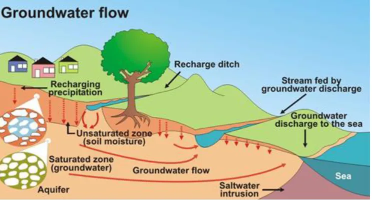
1.1 The hydrological cycle and groundwater flow 2

2.1 Hunk of bar of cross-sectional area A 9

3.1 Molecule diagram for Explicit method. 24

3.2 Mesh diagram of Explicit method 24

3.3 Mesh point of explicit method with h0.2 and 01

. 0  k

26

3.4 Molecule diagram for Implicit method 32

3.5 Mesh diagram for Implicit method 32

3.6 Mesh point Implicit method with h0.2 and 01

. 0  k

36

3.7 Molecule diagram for Crank-Nicolson Method 45

(12)

xiii

3.9 Mesh point Crank-Nicolson method with h0.2 and 01

. 0  k

49

4.1 Grid superimpose on the x-t plane. Point P is a typical node in the grid system with coordinates(x_i,t_j).

62

4.2 Mesh point of Explicit method with h10 and k 5 64

4.3 Mesh point of Implicit method with h10 and k 5 66

(13)

xiv

LIST OF ABBREVIATIONS

1-D - One-Dimensional

2-D - Two-Dimensional

3-D - Three-Dimensional

BEM - Boundary Element Method

FDM - Finite Difference Method

FEM - Finite Element Method

MQ-RBF - Multi-Quadric Radial Basis Function

(14)

xv

LIST OF SYMBOLS

h - Mesh size (step size for x)

k - Iteration parameters (step size for t) u (x, t) - Dependent variables

x, t - Independent variables a, b, c, d, e, f, g - Constant

t - Time

∆x, ∆t - Size of interval at x and t axis respectively

r - ratio

L - Length in x direction

(15)

xvi

LIST OF APPENDICES

Appendix Title Page

A Example 3.1 : Explicit method 79

B Example 3.2 : Implicit method 80

C Example 3.3 : Crank-Nicolson method 82

D

E

F

Example 4.1 : Explicit method

Example 4.2 : Implicit method

Example 4.3 : Crank-Nicolson method

85

86

(16)

1

CHAPTER 1

RESEARCH FRAMEWORK

1.1 Introduction

Mathematical problems can be solved analytically or numerically. However, analytic method scheme may be unsuccessful if the region of the problems is complex or the boundary conditions are time-dependent. In that case, numerical solution method will be very useful. The main goal in the field of numerical analysis is to provide compatible method in order to obtain the solutions to mathematical problems.

For scientific and engineering applications, it is often necessary to solve partial differential equations (PDE). Most partial differential equations for practical problems cannot be solved analytically. Therefore, numerical methods for partial differential equations are extremely important (Ya, Yan Lu).

(17)

2

in form and the solutions also related to the grid points (A. Thom and C. J. Apelt, 1961).

In this project, finite difference techniques; explicit method, implicit method and Crank-Nicolson method are applied for solving one dimensional heat equation and groundwater flow modeling.

1.2 Background of the Research

Groundwater is water located under the ground surface in soil pore spaces and in the fractures of rock formations (Adam Baharum et. al, 2009). A unit of rock or an unconsolidated deposit is called an aquifer when it can yield a usable quantity of water. The depth at which soil pore spaces or fractures and voids in rock become completely saturated with water is called the water table. Figure 1.1 shows the groundwater flow. Groundwater is recharged from, and eventually flows to the surface naturally; natural discharge often occurs at springs and seeps, and can form oases or wetlands. Groundwater is also often withdrawn for agricultural, municipal and industrial use by constructing and operating extraction wells. The study of the distribution and movement of groundwater is hydrogeology, also called groundwater hydrology.

(18)

3

Some of the established solution techniques available for solving the governing equations of the model are Finite Difference Method and Finite Element Method approximation or a combination of both provided that model parameters also initial and boundary conditions are properly specified. The numerical solution applied in this research work is the finite difference method. This is an old method made more useful with the advent of high performance computer systems.

1.3 Problem Statement

In this research, we investigate numerical solution for solving one dimensional heat equation and groundwater flow modeling using finite difference method such as explicit, implicit and Crank-Nicolson method manually and using MATLAB software.

1.4 Objectives of the Research

The specific objectives of this research are:

1. To solve one dimensional heat equation by using explicit finite difference method, implicit finite difference method and Crank-Nicolson method manually and using MATLAB software;

2. To derive one dimensional groundwater flow modeling;

3. To solve one dimensional groundwater flow modeling by using explicit finite difference method, implicit finite difference method and Crank-Nicolson method using MATLAB software.

(19)

4

1.5 Scope of Research

In recent years, a number of numerical methods have been introduced. This project is limited to solve one dimensional groundwater flow by using finite difference method. We will focus on three methods namely, explicit, implicit and Crank-Nicolson method.

1.6 Significant of the Study

(20)

5

1.7 Dissertation Report Organization

This research has been organized into five chapters. In chapter one, we discuss about the information of the whole research. This chapter introduced the background of the research, problem statement and the objectives for this research. Besides that, we have state the scope of research and the significance of the research. Lastly, we discuss on the organization of the report.

In chapter two, we discuss the literature review of this research. It give some review of previous work done by many researcher regarding for modeling of groundwater flow problem.

For chapter three, we explain about the algorithm of explicit, implicit and Crank-Nicolson method in order to solve the one dimensional of heat equation. We also give the example for all the methods. Additionally, we compare the results with exact solution.

In chapter four, we discuss the implementation of one dimensional groundwater flow modeling for explicit, implicit and Crank-Nicolson method. The problem we solve by using MATLAB software. Then, the results obtain are compared to each method and displayed in tables.

(21)

6

1.8 Research Methodology

SOLVING ONE DIMENSIONAL HEAT EQUATION AND GROUNDWATER FLOW MODELING USING FINITE DIFFERENCE METHOD

LITERATURE REVIEW: Search on the resources on this research topic. Include all type of resources such as books,

online sources, journals, articles and many more.

DESIGN THE STUDY AND DEVELOP THE

METHODS

Derive one dimensional heat equation.

Solving numerical method; explicit, implicit and Crank Nicolson method. Then, compare with analytical method (exact solution, Fourier Series)

Solve the problems by using MATLAB software.

DISCUSSION ON CASE STUDY

REPORT WRITING AND PRESENTATION

(22)

74

REFERENCES

[1] Ames, W. F. (1977). Numerical Methods for Partial Differential Equations. Academic Press New York.

[2] A Baharum, HF AlQahtani, Z Ali, H Lateh and KS Peng (2009). Modelling of Groundwater by Using Finite Difference Methods and Simulation. In: 10th Islamic Countries Conference On Statistical Science, Cairo, Egypt.

[3] A. Thom and C. J. Apelt (1961). Field Computations in Engineering and Physics. London: D. Van Nostrand.

[4] Che Rahim Che Teh (2013). Numerical Methods, Esktop Publisher.

[5] C. Babajimopoulos (1991). One-dimensional Unsaturated Flow in Soil. Volume 29, issue 2; 267–270.

[6] Daniel J. Duffy (2004). A Critique of the Crank Nicolson Scheme Strengths and Weaknesses for Financial Instrument Pricing. Datasim Component Technology BV.

[7] F.T. Tracy (2008). One-, two-, and three-dimensional solutions for counter-current steady-state two-phase subsurface ﬂow. International Journal of Multiphase Flow 34; 437– 446.

(23)

75

[9] Gerald W. Recktenwald (2004), “Finite-Diﬀerence Approximations to the Heat Equation.”

[10] Jim Douglas, Jr and Seongjai Kim (2000). On Accuracy of Alternating Direction Implicit Methods for Parabolic Equations.

[11] John Douglas Moore (2003) “Introduction to Partial Diﬀerential Equations.”

[12] L. Preziosi and A. Farina (2000). On Darcy’s Law for Growing Porous Media. International Journal of Non-Linear Mechanics 37 (2002); 485-491.

[13] Magnus. U. Igboekwe and N. J. Achi (2011). Finite difference method of modelling groundwater flow. Journal of water resource and protection, 192-198.

[14] Manoranjan V.S and Gomez M.O (2005). Alternating Direction Implicit (ADI) Method With Exponential Up Winding. Computers and Mathematics Application. Vol.3, No. 11, pp. 47-58.

[15] Mark M.Meerschaert and Charles Tadjeran (2004). Finite difference approximations for fractional advection–dispersion flow equations. Journal of Computational and Applied Mathematics 172; 65 – 77.

[16] Mategaonkar Meenal and T.I. Eldho (2011). Simulation of groundwater ﬂow in unconﬁned aquifer using meshfree point collocation method. Engineering Analysis with Boundary Elements 35, 700–707.

(24)

76

[18] Nur Ain Ayuni binti Sabri (2009). Solving Two-Dimensional Heat Equation Using Alternating Direct Implicit Method. B.Sc Thesis, Universiti Teknologi Malaysia.

[19] Nunzio Romano, Bruno Brunone and Alessandro Santini (1996). Numerical analysis of one-dimensional unsaturated flow in layered soils. Advances in Water Resources 21; 315-324.

[20] N. Mohankumar (2007). On the Numerical Solution of Radioactivity Migration in a Porous Medium. Annals of Nuclear Energy 34 ; 222–227.

[21] Pozrikidis C. (1998). Numerical Computation in Science and Engineering. Oxford University Press.

[22] P. Sochala, A. Ern and S. Piperno (2009). Mass conservative BDF-discontinuous Galerkin / explicit ﬁnite volume schemes for coupling subsurface and overland ﬂows. Comput. Methods Appl. Mech. Engrg. 198: 2122–2136.

[23] Pozrikidis C. (1998), Numerical Computation in Science and Engineering, Oxford University Press.

[24] Rectenwald G. W.(2004), “Finite-Difference Approximations to Heat Equations”.

[25] Remson, I., G. M. Hornberger and F. J. Molz (1971). Numerical Methods in Subsurface Hydrology. Wiley-Interscience, New York; 389 pp.

(25)

77

[27] S. Chen, F. Liu and K. Burrage (2013). Numerical Simulation of a New Two-Dimensional Variable-Order Fractional Percolation Equation in Non-Homogeneous Porous Media. Computers and Mathematics with Applications. In Press corrected proof.

[28] Soubhadra Sen, N. Mohankumar (2011). A computational strategy for radioactivity migration in a porous medium. Annals of Nuclear Energy 38; 2470–2474.

[29] S. Chen, F. Liu and K. Burrage (2013). Numerical Simulation of a New Two-Dimensional Variable-Order Fractional Percolation Equation in Non-Homogeneous Porous Media. Computers and Mathematics with Applications. In Press corrected proof.

[30] Stefan J. Kollet and Reed M. Maxwell (2006). Integrated surface– groundwater flow modeling: A free-surface overland flow boundary condition in a parallel groundwater flow model. Advances in Water Resources 29, 945–958.

[31] Thomas J.W. (1995), Numerical Partial Differential Equations, Springer.

[32] Tian Dongfang and Liu Defu (2011). A new integrated surface and subsurface ﬂows model and its veriﬁcation. Applied Mathematical Modelling 35, 3574–3586.

[33] Wang, H. F. and M. P. Anderson (1995). Introducing to groundwater modeling. Finite difference and finite element methods. Academic Press, 6277 Sea Harbor Dr. Orlando Florida 32887 USA, 1995, 237.

[34] Ya, Yan Lu “Numerical Methods for Differential Equations”.

(26)

78

[36] Zhen F. Tian (2010) A Rational High-Order Compact ADI Method For Unsteady Convection–Diffusion Equations. Computer Physics Communications 182; 649–662.

[37] Zhifeng Weng, Xinlong Feng and Pengzhan Huang (2012). A New Mixed ﬁnite Element Method Based on the Crank–Nicolson Scheme for the Parabolic Problems. Applied Mathematical Modelling 36; 5068–5079.