ZHANG, ZHE An Application of Linear Optimization in Anaglyph Stereo Image Render-ing. (Under the direction of Professor David F. McAllister).
by
Zhe Zhang
A thesis submitted to the Graduate Faculty of North Carolina State University
in partial fulfillment of the requirements for the Degree of
Master of Science
Operations Research
Raleigh
2006
Approved By:
Dr. S. Purushothaman Iyer
Biography
Acknowledgements
Contents
List of Figures vii
List of Tables viii
1 Introduction 1
1.1 Stereo Computer Graphics . . . 1
1.1.1 Depth Cues . . . 1
1.1.2 Stereoscopic Imaging . . . 3
1.2 Anaglyph Stereo Rendering . . . 4
1.3 Anaglyph Methods . . . 7
1.3.1 Color Spaces . . . 7
1.3.2 Background of Anaglyph Calculation Methods . . . 8
1.3.3 Photoshop and Modified Photoshop Algorithms . . . 10
1.3.4 Least Squares Algorithm . . . 11
2 Uniform Anaglyph Calculation 14 2.1 Uniform Calculation Algorithm . . . 14
2.1.1 A Revision of the LS Method . . . 14
2.1.2 Approximating in the Uniform Metric . . . 15
2.2 Background of Linear Programming . . . 16
2.2.1 Geometry of Linear Programming . . . 16
2.2.2 The Simplex Method . . . 19
2.2.3 Conclusion . . . 20
2.3 Color and Performance of the Uniform Method . . . 21
2.3.1 Color Test . . . 21
2.3.2 Color Results . . . 23
2.4 Computing Performances . . . 26
3 Accelerating the Calculation 27 3.1 Exploiting Color Coherence . . . 27
3.1.1 Color Coherence in Real World Images . . . 27
3.1.3 Processing Connected Regions with Low Costs . . . 34
3.2 Parallel Processing . . . 38
3.2.1 Parallelization without Color Coherence . . . 38
3.2.2 Parallelization and Color Coherence . . . 39
3.2.3 Load Balancing . . . 40
4 Acceleration Results 42 4.1 Results of Exploiting Color Coherence . . . 42
4.2 Results of Parallel Computing . . . 44
4.3 Conclusion . . . 46
5 Conclusion and Future Direction 48
Bibliography 49
Appendices 51
A Color Comparison Results 51
List of Figures
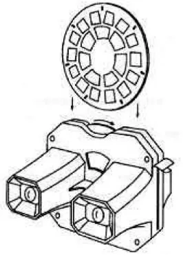
1.1 View-Master stereoscope . . . 5
1.2 Red/Cyan glasses transmission function . . . 6
1.3 Monitor spectral distributions . . . 6
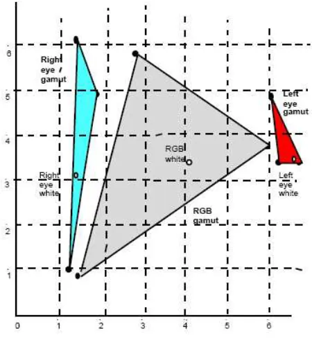
1.4 The CIE color space chromaticity diagram . . . 7
1.5 Gamuts in CIE space . . . 9
1.6 Images of equally spaced color points . . . 13
2.1 A vertex and a extreme point of a polyhedron . . . 18
2.2 The simplex algorithm . . . 19
2.3 Cube 6 - Stereo image rendered with different methods . . . 22
3.1 An example of color coherence . . . 28
3.2 A pixel’s neighbors . . . 29
3.3 Depth-first searching mechanism . . . 38
3.4 An extreme example . . . 40
4.1 A 203×305 pair of images . . . 43
4.2 A 230×261 pair of images . . . 43
4.3 A 1085×675 pair of images . . . 43
A.1 Cube 1 - Stereo image rendered with different methods . . . 52
A.2 Cube 2 - Stereo image rendered with different methods . . . 53
A.3 Cube 3 - Stereo image rendered with different methods . . . 54
A.4 Cube 4 - Stereo image rendered with different methods . . . 55
A.5 Cube 5 - Stereo image rendered with different methods . . . 56
A.6 Cube 6 - Stereo image rendered with different methods . . . 57
A.7 Cube 7 - Stereo image rendered with different methods . . . 58
A.8 Cube 8 - Stereo image rendered with different methods . . . 59
B.1 A 203×305 pair of images . . . 61
B.2 A 230×261 pair of images . . . 62
List of Tables
Chapter 1
Introduction
We present a new method for computing color anaglyph stereo images and discuss techniques to accelerate the calculation.
Stereo computer graphics and anaglyph image rendering concepts are introduced in chapter 1. Chapter 2 discusses in detail our new uniform anaglyph calculation methods. Also included in chapter 2 is a brief introduction to linear programming concepts and techniques. In chapter 3, we present a discussion of our efforts to accelerate the uniform calculation. The results of our acceleration techniques are given in chapter 4. Chapter 5 presents our conclusions and prospective research directions.
1.1
Stereo Computer Graphics
1.1.1 Depth Cues
The human visual system uses many depth cues to disambiguate the relative posi-tions of objects in a three-dimensional(3D) scene. These cues are divided into two categories: physiological and psychological([11]).
Physiological depth cues include the following:
a change in tension from the ciliary muscle. This depth cue is normally used by the visual system in tandem withconvergence.
Convergence. Convergence, or simplyvergence, is the inward rotation of the eyes to converge on objects as they move closer to the observer.
Binocular disparity. Binocular disparityis the difference in the images projected on the left and right eye retinas in the viewing of a 3D scene. It is the salient depth cue used by the visual system to produce the sensation of depth, orstereopsis. Any 3D display device must be able to produce a left and right eye view and present them to the appropriate eye separately. There are many ways to do this as we will see below.
Motion parallax. Motion parallax provides different views of a scene in response to movement of the scene or the viewer. Consider a cloud of discrete points in space in which all points are the same color and approximately the same size. Because no other depth cues (other than binocular disparity) can be used to determine the relative depths of the points, we move our head from side to side to get several different views of the scene (called look around). We determine relative depths by noticing how much two points move relative to each other: as we move our head from left to right or up and down; the points closer to us appear to move more than points further away.
Psychological depth cues include the following:
Linear perspective. Linear perspective refers to the change in image size of an object on the retina in inverse proportion to the objects change in distance. Parallel lines moving away from the viewer, like the rails of a train track, converge to a vanishing point. As an object moves further away, its image becomes smaller, an effect called perspective foreshortening. This is a component of the depth cue of retinal image size.
Shading and shadowing. The amount of light from a light source illuminating a surface is inversely proportional to the square of the distance from the light source to the surface. Hence, surfaces of an object that are further from the light source are darker (shading), which gives cues of both depth and shape. Shadows cast by one object on another (shadowing) also give cues to relative position and size.
Retinal image size. We use our knowledge of the world, linear perspective, and the relative sizes of objects to determine relative depth. If we view a picture in which an elephant is the same size as a human, we assume that the elephant is further away since we know that elephants are larger that humans.
Texture gradient. We can perceive detail more easily in objects that are closer to us. As objects become more distant, the texture becomes blurred. Texture in brick, stone, or sand, for example, is coarse in the foreground and grows finer as the distance increases.
Color. The fluids in the eye refract different wavelengths at different angles. Hence, objects of the same shape and size and at the same distance from the viewer often appear to be at different depths because of differences in color. In addition, bright-colored objects will appear to be closer than dark-colored objects.
The human visual system uses all of these depth cues to determine relative depths in a scene. In general, depth cues are additive; the more cues, the better able the viewer is to determine depth. However, binocular disparity, accommodation, and convergence are generally considered as the three most powerful cues for determining relative depth. While it is accepted by most people that binocular disparity is more important as a depth cue than accommodation and convergence, the latter two do influence depth perception when coupled with binocular disparity, especially for observer distances less than 2 meters([9]).
1.1.2 Stereoscopic Imaging
Most 3D displays fit into one or more of three broad categories: holographic,
multiplanar, andstereo pair([11]). In general, holographic and multiplanar images produce “real” or “solid” images, in which binocular disparity, accommodation, and convergence are consistent with the apparent depth in the image.
from different positions relative to the scene([11]).
The computation of stereo pairs is discussed in detail in Chapter 5 of [11] and we will not cover that part here. After stereo pairs are computed, a mechanism is required in viewing them so that the left eye sees only the left eye view and the right eye sees only the right eye view([12]). It is common in display technologies to use a single screen to reflect or display both images either simultaneously (time parallel) or in sequence (time multiplexed or field sequential).
In the field-sequential or time multiplexed technique, the left/right views are alter-nated on the display device, and a blocking mechanism to prevent the left eye from seeing the right eye view and vice versa is required. While older technologies used mechanical devices to occlude the appropriate eye view during display refresh, newer technologies use electro-optical methods such as liquid-crystal plates. These techniques fall into two groups: those that use active vs. passive viewing glasses.
Time-parallel methods present both eye views to the viewer simultaneously and use optical techniques to direct each view to the appropriate eye. The View-Master, illustrated in Figure 1.1, is an example of time-parallel displays devices. The View-Master stereoscope uses two separate optical systems. Each eye looks though a magnifying lens to view a slide. The slides are taken with a pair of cameras mounted on a base, replicating the way we see the world with two eyes ([11]). Anaglyph, discussed in detail in section 1.2 below, is another popular time-parallel method.
1.2
Anaglyph Stereo Rendering
Figure 1.1: View-Master stereoscope
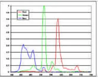
anaglyph filters are shown in Figure 1.2.
A significant problem of the anaglyph method is a phenomenon calledghosting or
cross talk. It is caused by the fact that the filters do not completely eliminate the opposite-eye view, so that the left opposite-eye saw not only its image but sometimes part of the right-opposite-eye image as well. In this case the image can appear blurred or a second or double image appears in regions of the scene being viewed. If we observe Figure 1.2 we will find that colors with wavelengths between 550 and 600 are passed by both filters and hence ghosting will occur for colors in the region.
Another problem is that the colors seen through each filter are often not repre-sentable by the display device and hence a phenomenon called retinal rivalry or binocular rivalry will occur. Retinal rivalry refers to the fact that when the color disparity between the left- and right-eye views is very large, objects appear double, with two monocular im-ages striking corresponding regions of the retinas. A more detailed discussion about retinal rivalry can be found in chapter 4 of [11].
(a) Left eye transmission function - Red fil-ter
(b) Right eye transmission function - Cyan filter
Figure 1.2: Red/Cyan glasses transmission function
(a) CRT monitor primary distributions (b) LCD monitor primary distributions
Figure 1.3: Monitor spectral distributions
of the pixel in the anaglyph image. Thus it is difficult, or impossible, to represent the same amount of information contained in the two original images.
We will see in section 2.3 that all the three issues mentioned above is evident in some of the color examples, especially those produced by the existing anaglyph methods.
Figure 1.4: The CIE color space chromaticity diagram
1.3
Anaglyph Methods
In this section we will introduce the background(1.3.2) and several different methods(1.3.3 and 1.3.4) for producing anaglyph stereo images, which were summarized and studied by Sanders and McAllister in [14].
1.3.1 Color Spaces
Our discussion below will concern two distinct color systems. TheRGB additive color system, which is used by most computer monitors and storage systems, produces colors by representing each of them as a linear combination of red, blue, and green.
Another color system is called theCIE, named after Commission Internationale de l’Eclairage, the French-language name for the International Commission on Illumination. The CIE color system characterizes colors by a luminance parameter Y and two color coordinates x and y which specify the point on the chromaticity diagram shown in Figure 1.4.
The original left- and right-eye views are represented in the RGB system. In the
2 we will convert the colors into the CIE space, because the colors that can be seen through the filters, in particular those that are produced by monitors, are not representable in the RGB space, as can be observed from Figure 1.5.
1.3.2 Background of Anaglyph Calculation Methods
The set of representable colors or the color solid on a display using the RGB color system is the unit RGB cube (3- cube). The cube lies in the 3 dimensional vector space R3. The basis or primaries are the colors red, green and blue.
The “anaglyph RGB color solid” in the six dimensional vector spaceR6 is a unit hypercube (6-cube) with 64 vertices corresponding to the RGB corners of the cube inR3 for the left and right eyes. Counting base 2 we can order the vertices of the 6-cube: [0,0,0,0,0,0] = [black, black], [0,0,0,0,0,1] = [black, blue],. . ., [1,1,1,1,1,1] = [white, white]. Anaglyph methods compute a map from the 6-cube in R6 to R3. We can examine the order and placement of the image of the 6- cube vertices to gain understanding of the method.
Three of the algorithms we analyze are linear; there is a 3×6 matrix representation of the map from R6 to R3 in each case. We define v = [rl, gl, bl, rr, gr, br]T which are the RGB coordinates of the left and right eye color channels. The linear algorithms compute [r, g, b]T = Bv. The linear methods differ only in the matrix B used to compute the map.
If a method produces colors that are not representable on the display (a coordinate lies outside the interval [0, 1]), clipping (projection) is used. Clipping maps nonrepresentable colors to the surface of the 3-cube. A projection map is linear.
Region merging occurs when adjacent regions of different colors are mapped to the same anaglyph color. This can affect depth and detail perceived in stereo images[13]. We note that clipping can cause region merging.
The spectral distributions of the phosphors on CRTs are shown in Figure 1.3(a). They have been uniformly scaled so the maximum value of red is 1. We also include the spectral distributions of the primaries for LCD monitors in Figure 1.3(b).
CCRT =
XR XG XB
YR YG YB
ZR ZG ZB
=
11.6638 8.3959 4.65843 7.10807 16.6845 2.45008
.527874 3.79124 24.0604
and
CLCD =
XR XG XB
YR YG YB
ZR ZG ZB
=
0.4243 0.3105 0.1657 0.2492 0.6419 0.1089 0.0265 0.1225 0.8614
The discussions below are focused on LCD displays, so in the following discussion we let the conversion matrixC =CLCD.
The gamut (on the CIE chromaticity diagram) for the spectral distributions of CRT monitors given in Figure1.3(a) is the RGB triangle in Figure1.5. The spectral distributions of CRT monitors have a similar gamut.
1.3.3 Photoshop and Modified Photoshop Algorithms
In the original Photoshop algorithm [17] (PS) the red channel of the left eye view becomes the red channel of the anaglyph and vice versa for the blue and green channels of the right eye. This is equivalent to projecting the left eye RGB point to the red axis of the RGB cube (setting the G and B channels to zero) and the right eye RGB point to the GB plane (thus setting the red channel to zero). See Figure 8. The two resulting vectors are added to compute the color of the pixel in the anaglyph. This method is linear. The matrix B is
B=
1 0 0 0 0 0 0 0 0 0 1 0 0 0 0 0 0 1
The algorithm ignores the transmission function of the glasses, which means the computed anaglyph is the same for all filters. Another observation is that all colors with the same left eye red channel and the same blue/green channels in the right eye view will be mapped to the same color.
As a variant of the PS method, the modified photoshop algorithm (MPS) converts the left eye image to grayscale first and then projects as described above. If we use a linear grayscale conversion algorithm (such as the NTSC luminance standard where grayscale = .299r + .587g + .114b [3]) we premultiply v by a partitioned matrix of the form
G 0 0 I
where I is the 3x3 identity and G is the matrixG=
α1 α1 α1
0 1 0
0 0 1
where the αi’ s are
nonnegative, sum to 1, and are the coefficients that convert the red channel to grayscale. We then apply the matrix B above. This gives the new matrix
B=
α1 α2 α3 0 0 0
0 0 0 0 1 0
0 0 0 0 0 1
1.3.4 Least Squares Algorithm
While the PS and MPS methods ignore the transmission properties of the filters, actually the colors visible through a filter depend on the transmission function f(λ) of the filter. As discussed in section 1.2, the function f specifies the percentages of each visible wavelength λ transmitted by the filter. The product of the primary spectral distribution with the transmission function gives the spectral distribution of the primary as seen through the filter. The matrices Al for the left eye and Ar for the right eye convert the resulting filtered colors to CIE coordinates. For some common red/cyan glasses used below, these conversion matrices are:
Al=
0.1840 0.0179 0.0048 0.0876 0.0118 0.0018 0.0005 0.0012 0.0159
, Ar=
0.0153 0.1092 0.1171 0.0176 0.3088 0.0777 0.0201 0.1016 0.6546
In[5] Eric Dubois showed how to use the transmission properties and spectral distributions for approximating colors in CIE color space to compute anaglyph colors. Dubois defined the length of a vector x = [X, Y, Z] in CIE space, using the Euclidean norm, kxk2 = (X2+Y2+Z2)
1
2. The distance between two points x1 and x2 is therefore kx1−x2k2. In this case determining the closest vector in a subspace to a point not in the subspace is called least squares approximation (LS); the CIE color space is a linear space and approximation can be accomplished by a simple matrix multiplication for each pixel. LS approximation is equivalent to a projection inR6 to the 3D subspace spanned by the 6 dimensional columns of the partitioned 6 x 3 matrix R defined below with right hand side partitioned vector d. The matrix C is the RGB-CIE conversion matrix defined above and
v is the 6 component vector consisting of the left eye RGB colorCLand the right eye color
CR, v= [CL, CR]T:
R= Al Ar
, d=
C 0
0 C
v (1.1)
The projection minimizes the Euclidean length of the vector R[r, g, b]T −d.
w3 = [1,1,1]T in R3 is mapped to the white/white vector w6 = [1,1,1,1,1,1]T in R6. The linear map can be written as [r, g, b]T = N(RTR)−1RTd =Bv. The diagonal matrix
N can be computed from the equation wT3 = N(RTR)−1RTwT
6. The B matrices for LS approximation is
B =
0.4154 0.4710 0.1669 −0.0109 −0.0364 −0.0060 −0.0458 −0.0484 −0.0257 0.3756 0.7333 0.0111 −0.0547 −0.0615 0.0128 −0.0651 −0.1287 1.2971
We note that the approximation may result in RGB components that are out of range. That is, some may be negative and some may exceed 1. Dubois recommends clipping to the RGB unit cube to solve this problem. Although this process involves a trivial computation, applying it to every pixel in an image adds to the time complexity. In addition, the method produces images that can be a bit dark. It does not preserve color equality as the Photoshop method does. That is, ifCL=CR, it is not necessarily the case that the optimal solution is [r, g, b]T =CL. In Figure 1.6(a) we have chosen equally spaced colors in the RGB cube forCL=CR. Figure1.6(b) shows the optimal solutions in the RGB cube. Note how the solutions have been mapped to a parallelepiped and many lie outside the unit RGB cube.
Greyscale, however, is preserved in the sense that if v is a (nonnegative) scalar multiple of white, v = αW, then the optimal solution is also a scalar multiple of white. This follows from the properties of norms and the fact that matrix multiplication is linear:
(a) Equally spaced colors in RGB (b) Images of points in part (a)
Chapter 2
Uniform Anaglyph Calculation
2.1
Uniform Calculation Algorithm
2.1.1 A Revision of the LS Method
Another way to view the problem of anaglyph calculation is to consider it as trying to solve a system of equations. For each pixel of an anaglyph there are three unknowns to be calculated, namely the red, green, and blue values of the color at that pixel. The constraints to be satisfied are the red, green, and blue values that should be transmitted to the left and right eyes of the viewer through the filters. Recall from section 1.3.4 that if the red, green, and blue values at a pixel of an anaglyph are represented as a vector [r, g, b]T, then the colors seen through the filters are described by the 6 dimensional vectorR[r, g, b]T; the colors that the left and right eyes of a viewer should see are described by the vector d where matrixR and vector d are defined in equation 1.1.
The goal of anaglyph calculation is to findr, g, b values such that:
R[r, g, b]T =d (2.1)
we can see that LS method actually tries to determine a vector in the range space of matrix
R that is closest to the pointd. That is equivalent to calculating the least squares solution of the system, and can be done by pre-multiplying the right-hand side vector d with the Moore-Penrose pseudoinverse of matrixR (scaled by the matrix N so that the white vector inR6 is mapped to the white vector inR3).
2.1.2 Approximating in the Uniform Metric
Based on the LS method, we attempt to produce better color results by calculating approximate solutions to the system in Equation 2.1 using another metric. Thus we change the length measure or the norm to the Chebychev, minimax, infinity oruniform norm of a vector x and define kxk∞ = max{|X|,|Y|,|Z|}. Approximation is in CIE space as in the
Dubois calculation but we minimize the length of the vectorR[r, g, b]T−dusing the uniform norm (UN) instead.
Using the uniform metric in this problem has an intuitive advantage compared with using the Euclidean metric. The 6 equations in the linear system in Equation 2.1 represent the relations between the red, green, and blue values the viewer’s left and right eye should see and the values that his/her left and right eyes actually see when viewing an anaglyph through filters. While the LS method minimizes the square-sum of the 6 differences between the ideal values and the actual values, the UN method minimizes the maximal value among those 6 differences. Thus if we use the UN method, the total error will be more evenly distributed among the 6 equations.
As in the LS case, we want to ensure that the white vectorw3 = [1,1,1]T inR3 is mapped to the white/white vector w6 = [1,1,1,1,1,1]T in R6. Instead of normalizing in the RGB space as the LS method does, we normalize in the CIE space. In other words, we compute the diagonal normalization matrixN such that Rw3 =N w6, which givesN = Diag[6.60522, 3.23678, 0.00263908, 4.02254, 8.12129, 12.624]. To minimize the maximum deviation, we use a 7th variable and we formulate the approximation problem as a linear programming problem (LP), which will be studied in more detail in section 2.2:
minimize subject to the constraints(s.t.) : (2.2) |(R[r, g, b]T −N d)i| ≤,1≤i≤6
The simplex method for solving LPs, which will be introduced in section 2.2.2, computes only nonnegative solutions. Sinceis bounded below automatically, the problem becomes a 7-variable LP with 15 constraints (the absolute value constraints are converted to two constraints each).
We can write the constraints as follows:
minimize subject to the constraints(s.t.) : (2.3) −≤R[r, g, b]T −N d)
i ≤,1≤i≤6
r, g, b ≤1 where all variables are nonnegative.
As in the LS case it does not preserve color equality. The bounds on r, g, and b prevent us from using the same argument as in the LS case, but numerical experiments suggest that it does preserve greyscale.
2.2
Background of Linear Programming
As stated above, Equation 2.2 is alinear programming problem (LP). According to [2],linear programming is the problem of minimizing a linear cost function subject to linear equality and inequality constraints. A general linear programming problem can always be transformed into an equivalent problem in the following form:
minimize cTx s.t. (2.4)
Ax≤b x unrestricted
In the following sections (2.2.1, 2.2.2 and 2.2.3) we will introduce concepts and methods for solving LPs. For the convenience of discussion we assume that the matrix A always has linearly independent rows.
2.2.1 Geometry of Linear Programming
Definition 2.2.1 Apolyhedronis a set that can be described in the form {x∈ <n|Ax≤
b}, where A is an m×n matrix and bis a vector in <m.
According to Definition 2.2.1 it can be seen that the feasible region of an LP in the form 2.4, i.e., the set of all points x that satisfy the constraint functions Ax ≤ b, is a polyhedron. It is observed from simple LP examples that the optimal solutions are always obtained at the “corners” of the feasible regions, which are polyhedra. In order to establish this fact, first we need the mathematical definition of “corners” of polyhedra. Two important geometric concepts,extreme points and vertices [2], are defined below.
Definition 2.2.2 Let P be a polyhedron. A vector x∈P is an extreme point of P if we
cannot find two vectors y,z ∈ P, both different from x, and a scalar λ ∈ [0,1], such that
x=λy+ (1−λ)z.
An example is shown in Figure 2.1(a). For any two points y and z in the polyhe-dron, x is not on the line segment that joins them, in other words, x is an extreme point of the polyhedron.
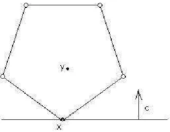
Definition 2.2.3 Let P be a polyhedron. A vector x ∈ P is a vertex of P if there exists
some vector c such that cT x< cT y for all y satisfying y∈P andy6=x.
In view of the above definition, the point x in Figure 2.1(b) is a vertex of the polyhedron, because for the vector c shown in this figure, cTx < cTy for any point y 6= x in the polyhedron.
To establish the relation between optimal solutions and “corners” of polyhedra, we also need to introduce the concept ofbasic feasible solutions (BFS) [2] of an LP as follows:
Definition 2.2.4 Consider a polyhedron P defined by linear equality and inequality
con-straints, and let x* be an element of <n. We say an equality constraint is active if it is
satisfied (holds); we say an inequality constraint is active if it is satisfied and the
(a) Extreme point (b) Vertex
Figure 2.1: A vertex and a extreme point of a polyhedron
(a) The vector x* is a basic solutionif:
(i) All equality constraints are active;
(ii) Out of the constraints that are active at x*, there are n of them that are linearly
independent.
(b) If x* is a basic solution that satisfies all of the constraints, we say that it is a basic
feasible solution.
2.2.2 The Simplex Method
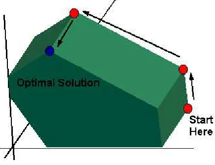
A common approach for solving an LP is the simplex method. The simplex method is based on the conclusion we made in section 2.2.1 and searches for an optimal solution by moving from one basic feasible solution to another, along the edges of the feasible set, always in a cost reducing direction [2]. Figure 2.2[4] gives a simple illustration of how the simplex method works, where the green area is the feasible region.
Figure 2.2: The simplex algorithm
In order to develop and implement the simplex method, we need to introduce the procedure of constructing basic feasible solutions and the mechanism of moving from one basic feasible solution to another with reduced cost. First we need to introduce the following standard form for an LP:
minimize cTx s.t. (2.5)
Ax=b x≥0
As argued in [2], any LP in form 2.4 can be further converted to the above standard form. Furthermore, according to the following theorem from [2], we can construct all basic feasible solutions of an LP in standard form 2.5 with simple algebraic operations:
matrix A has linearly independent rows. A vector x∈ <n is a basic solution if and only if
we have Ax=b, and there exist indicesB(1), . . . , B(m) such that:
(a) The columns AB(1), . . . ,AB(m) are linearly independent;
(b) If i6=B(1), . . . , B(m), then xi = 0.
In view of the above theorem, all basic solutions to a standard form LP can be constructed by first choosing m linearly independent columnsAB(1), . . . ,AB(m), then letting
xi = 0 for all i 6= B(1), . . . , B(m) and finally solving the system of m equations Ax = b for the unknowns xB(1), . . . ,xB(m). If the basic solution constructed has all nonnegative components, then it is a basic feasible solution. The set of columnsB={AB(1), . . . ,AB(m)} forms a basis for the m dimensional linear space and is called the as the basis of the corresponding basic solution.
The simplex method moves from one basic feasible solution to another by taking one column out of the current basis and inserting a new column into it. If two bases are the different only for one column, then they are said to be adjacent bases and the corresponding basic feasible solutions are also said to be adjacent. Adjacent basic feasible solutions correspond to adjacent vertices of the feasible region of the LP. Thus the simplex method moves from one vertex to an adjacent one with reduced cost. If all adjacent vertices are with higher costs than the current one, then the optimum is achieved. An anti-circling scheme is used so that the algorithm will never consider a previously visited vertex. This scheme, combined with the fact that there are always finite number of vertices in the polygon, guarantees that the simplex algorithm finds the optimum in a finite number of steps.
2.2.3 Conclusion
important example is the interior point method introduced in [10]. Instead of moving from one vertex to another along edges like the simplex algorithm, the interior method goes through the interior of the polyhedral feasible region to find the optimal solution.
While the interior algorithm has a better asymptotic complexity, the simplex algo-rithm has less cost for a single step. In our problem the small size of the LP justifies using the simplex algorithm. However, as we will discuss in chapter 5, applying the interior point method has a potential of bringing about a further acceleration of the calculation, and it is a direction of our future research.
Generally speaking, solving an LP is considerably more computationally complex than applying a single matrix multiplication. Hence the problem produces interesting com-putational issues and in section 3 we seek parallel computation methods to accelerate the calculation to take advantage of coherence in digital images: the optimal solution at a given pixel is normally close to the optimal solutions of the surrounding pixels and the optimal solution for a pixel in a given frame of video is usually close to the optimal solution in the succeeding frame. Our goal is to produce anaglyphs of video signals at NTSC rates so we can apply the technique to problems like distance learning and virtual laboratories.
2.3
Color and Performance of the Uniform Method
2.3.1 Color Test
We compare the color, brightness and ghosting qualities of four algorithms: UN, LS, PS, and MPS. We created Gouraud shaded ellipsoids using 3D Studio. The hue and saturation over a given ellipsoid are the same for all pixels, but brightness varies from approximately 0 to 100 percent.
All ellipsoids are about the same size and the same distance from the viewer. We chose 64 RGB values that were equally spaced over the RGB cube, grouping them eight at a time. The colors are the coordinates of vertices of subcubes with edge lengths approximately
255
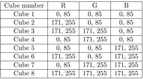
3 ∼= 85. We consider all permutations of the intensities of 0, 85, 171 and 255 taken 3 at a time. The background is set to a neutral gray intensity of 166. There is no gamma correction. The cubes are numbered as shown in Table 2.1:
(a) LS (b) MPS
(c) UN (d) PS
(e) Left eye view with true color
Table 2.1: Cube numbering scheme
Cube number R G B
Cube 1 0, 85 0, 85 0, 85
Cube 2 171, 255 0, 85 0, 85 Cube 3 171, 255 171, 255 0, 85 Cube 4 0, 85 171, 255 0, 85
Cube 5 0, 85 0, 85 171, 255
Cube 6 171, 255 0, 85 171, 255 Cube 7 0, 85 171, 255 171, 255 Cube 8 171, 255 171, 255 171, 255
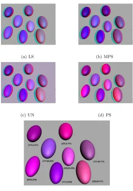
cubes are given in Appendix A. We note for cube 6 the significant color differences produced by the methods when viewed without using anaglyph filters
2.3.2 Color Results
We did not attempt to perform a study in which the results were statistically significant since the effect of retinal rivalry cannot be predicted nor controlled. However, the comparisons for three non-colorblind observers were consistent, so we report them here. We compare each ellipsoid with the original left or right eye viewwith glasses (we note that comparing colors without the glasses is pointless and can result in misleading conclusions). We used three different pairs of red/cyan glasses: Reel3-D No. 7003, IMAX Fujitsu and the glasses provided by ABC to view the television showMedium. The results were independent of the glasses.
value of R in the anaglyph making the image darker. This phenomenon is evident in the results for Cube 2.
For cube 1 (Figure A.1), the point (0,0,0) or black, is the same for all methods, as was (0, 0, 85). UN is the best at points (85,0,0) and (85,0,85). PS is slightly worse, with MPS and LS equally bad. For (85,85,0), LS is only slightly better than MPS, and UN and PS are equally poor. LS is again the best for (0,85,0), then UN, then PS, and finally MPS. At (0,85,85) UN and LS are equally bad, and MPS is the worst. All are similar for the gray level (85,85,85) although UN is slightly darker.
For cube 2 (Figure A.2), shades of red, UN is best for all points. However, UN, while being a similar hue, is too bright, and there is conspicuous ghosting. LS and MPS are always too dark, but at points (171,0,0), (171, 85,85) and (255,0,0), LS is the worst, while MPS is worst at (255,0,85), (255,85,85), (171,0,85), and (255,85,0). MPS and LS are similar at (171,85,0). Retinal rivalry is a problem for PS.
Color cube 3 (Figure A.3) contains pale oranges and greens. The results are varied. At (171,171,0) UN is a similar hue, but too light. MPS is next in accuracy and LS worst. At (255,171,0), UN is again too bright, then LS, and MPS. UN, PS and MPS are equal, and LS is worst at (171,171,85) and (171,255,85). LS is best at (171,255,0), then MPS, and UN last. LS and MPS are almost the same at (255,255,0), and UN is the worst. At (255,171,85), UN is the best, followed by LS, then MPS. UN is consistently too light, but the hues are closer to the originals than the hues of MPS or LS.
Cube 4 (Figure A.4) is shades of green. UN is the best at (0,171,0). PS is sec-ond, MPS is too light, and LS is too dark. For the points (0,255,0), (85,171,0),(85,255,0), (0,171,85), (0,255,85), (85,171,85), and (85, 255,85), there is a large amount of ghosting and retinal rivalry in PS. UN is consistently second best for these points, with a slightly different hue, but with the least ghosting and retinal rivalry. MPS is third with a different hue and too light. LS is worst with a much darker intensity and a different hue.
second, then LS, and then MPS. PS is again the closest at (85,85,171), followed by MPS. UN and LS are equally too light and the wrong hue. The worst ghosting takes place at (0,0,255), with MPS best and the others almost impossible to see because of the retinal rivalry.
Cube 6 (Figure 2.3) contains the purple hues. UN is best for most cases. UN is best for (171,85,171) and (171,85,255), followed by PS which has more ghosting. LS and MPS were too dark, but MPS was the darkest. For the remaining points the order in decreasing hue approximation is UN, LS and MPS. For these remaining points there is significant retinal rivalry in PS. There is less retinal rivalry and ghosting is least for UN.
Cube 7 (Figure A.7) is the cyan region. There is considerable ghosting and retinal rivalry in PS. Second is MPS, with the right hue, but too light. LS is always the wrong hue, but the best brightness match. UN is consistently too dark and the wrong hue.
Cube 8 (Figure A.8) is the white corner of the RGB cube, the least saturated colors. All the methods produce approximately the same image for (171,171,171) and (255,255,255). All produce images of equal brightness at (171,171,255), but UN has a distinct rim in the ghosting area, an interesting phenomenon. At (171,255,171) LS is the wrong hue, MPS is worse, and UN is the worst but has the least amount of ghosting. UN is best at (255,171,171). LS is the wrong hue, and MPS is too dark and the wrong hue. At (255,255,171), MPS is best. LS is too bright, and UN is far too bright. There is considerable retinal rivalry in the PS approximation at (255,171,255), but it is the best hue approximation. UN and LS are about equal, and MPS is too dark. At (171,255,255) none of the three methods produces the correct hue. MPS is far too light, and UN is too dark.
2.4
Computing Performances
As expected in section 2.2.3, the computation of UN method takes much more time than that of PS, MPS and LS methods. When we implement the calculation with Mathematica, it takes more than 3 hours to process a 1085×675 image on a Dell 700m laptop computer with a 1.6 GHz CPU and 512 M memory. The implementation in C++ language is much faster, but it still takes more than 2 minutes to process the same image. After testing the UN method on a set of images with different sizes, from 60030 to 856544 pixels, we find that the processing time is 1.5×10⁻⁴ to 2.5×10⁻⁴ seconds per pixel, the average being 1.9×10⁻⁴ seconds.
Chapter 3
Accelerating the Calculation
In the discussion below, the conclusions are based on the behavior of our methods for several continuous tone photographs. Our computing environment for the uniprocessor case is a Dell 700m computer with 1.6 GHz CPU. Our parallel processing environment is an 8-node Cluster, where each node has dual 2.8-3.06 GHz processors. More specific information about the experimental environments and results can be found in section 4.
As stated in chapter 2, UN calculation is considerably more expensive computa-tionally than the methods PS, MPS and LS, where only matrix multiplications are required. A stereo pair of 1085 by 675 images we test requires the unaccelerated UN method 127 sec-onds to render the anaglyph while the PS method requires less than 0.01 second. Our efforts to accelerate the UN calculation is described in the following sections.
3.1
Exploiting Color Coherence
3.1.1 Color Coherence in Real World Images
Figure 3.1: An example of color coherence
visited, so that future accesses are likely to find the desired data in the Cache.
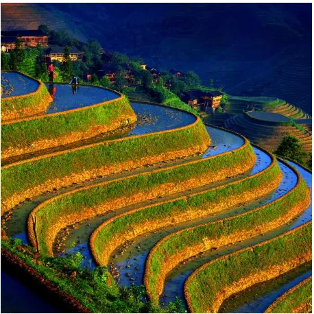
As mentioned in [6], in computer graphics and image compression there are also many forms of coherence that are used to make rendering more efficient. In our case the color of a pixel is often similar to that of its neighbors, where being similar is defined as being close relative to a distance measure or metric in the color space being considered. Furthermore, there often exist sets of pixels with similar colors, and located as connected regions (defined below) in the image. An example is shown in Figure 3.1.
In our discussion an image is viewed as a 2D array of pixels. For a pixelq which lies in the ith row and the jth column, another pixel p is q’s neighbor if p’s row index is
i−1, i, or i+ 1, andp’s column index is j−1,j, or j+ 1. As shown in Figure 3.2, pixel
q has 8 neighbors, namely p1, p2, . . . , p8. A set S of pixels forms a connected region if for any two pixels p0, pn∈S, there exist pixels p1, p2, . . . , pn−1 ∈S such that pi is a neighbor of pi+1 fori= 0,1, . . . , n−1.
Figure 3.2: A pixel’s neighbors
Semantic objects in an image do not generally have regular shapes, but in most cases each object occupies a connected region in the image. One example is the terraced field in Figure 3.1, where each terrace, although in very irregular shape, is a connected region with similar colors.
With the definition of connected regions we are able to recognize semantic objects and divide pixels with similar colors into groups. In section 3.1.3 an approach is developed to take each connected region with similar colors as a unit, solve an LP for each unit just once, and process all the pixels in the unit with matrix-vector multiplications.
3.1.2 Color Coherence and Linear Programming
Intuitively two pixels have close colors implies that the optimal solutions of the associated LPs should be “close” in the sense that solutions will often be the same or “adjacent” on the simplex defining the set of feasible solutions. We seek to find ways to exploit this in the simplex algorithm: after solving the LP for one pixel we try to use the solution to help process its neighbors faster, instead of executing the simplex algorithm for every pixel.
constraints when put in the standard form (2.5).
Moreover, according to Theorem 3.1.1 from [2], if the difference between each component of the right hand sides of two such problems is within a certain interval (specified below), and we have already computed the solution to one of the problems, then the other can be solved with a simple matrix-vector multiplication.
Theorem 3.1.1 Let B be the basis of the current optimal solution, andg= (β1i, β2i, . . . , βmi)
be the ith column ofB−1. Suppose that the ith component bi of the right hand side vector b
is changed to bi+δ, and δ satisfies:
max
{j|βji>0}
(−xB(j)
βji
)≤δ≤ min
{j|βji<0}
(−xB(j)
βji )
For δ in this range, the new optimal solution has the same optimal basis as the old one, and
the value is given by cTBB−1(b+δei), wherec is the cost vector introduced in Equations 2.4
and 2.5, and cB = (cB(A), cB(2), . . . , cB(m)) with B(1), B(2), . . . , B(m) being the indices of
the current basis.
In our specific problem the difference between the right hand sides of two linear programming problems depends on the difference between the colors of the two correspond-ing pixels. Thus if two pixels have similar colors, their associated LPs have the same optimal basis.
We use a numerical example to illustrate this. For a pixel with left eye color (rl, gl, bl) and right eye color (rr, gr, br), the linear programming problem is given by:
minimize s.t
−≤R[r, g, b]−N d)i ≤,1≤i≤6
r, g, b≤1,
where d =
C 0
0 C
·[rl, gl, bl, rr, gr, br]T. In order to apply the simplex algorithm, we
LP has 15 inequality constraints and 4 variables , r, g, andb. We denote , r, g, andb by
x1, x2, x3, andx4, respectively. For each inequality equationα1x1+α2x2+α3x3+α4x4 ≤b, if we introduce a slack variable xs which is restricted to be nonnegative, we can get the equivalent formα1x1+α2x2+α3x3+α4x4+xs =b, xs ≥0. Thus by introducing one slack variable for each inequality, the LP can be transformed into the the standard form given below:
minimize x1 s.t. (3.1)
E[x1, x2, x3, x4, x5, . . . , x19]T = F[rl, gl, bl, rr, gr, br,1,0,0]T
x1, x2, x3, x4, x5, . . . , x19≥0 The matrices E and F are given below:
E=
−1 −5.423 −0.807 −0.047 1 0 0 0 0 0 0 0 0 0 0 0 0 0 0
−1 −2.710 −0.502 −0.025 0 1 0 0 0 0 0 0 0 0 0 0 0 0 0
−1 −0.00006 −0.0004 −0.002 0 0 1 0 0 0 0 0 0 0 0 0 0 0 0
−1 −0.180 −1.640 −2.003 0 0 0 1 0 0 0 0 0 0 0 0 0 0 0
−1 −0.448 −6.315 −1.358 0 0 0 0 1 0 0 0 0 0 0 0 0 0 0
−1 −0.289 −2.393 −11.062 0 0 0 0 0 1 0 0 0 0 0 0 0 0 0
−1 5.423 0.807 0.047 0 0 0 0 0 0 1 0 0 0 0 0 0 0 0
−1 2.710 0.502 0.025 0 0 0 0 0 0 0 1 0 0 0 0 0 0 0
−1 0.00006 0.0004 0.002 0 0 0 0 0 0 0 0 1 0 0 0 0 0 0
−1 0.180 1.640 2.003 0 0 0 0 0 0 0 0 0 1 0 0 0 0 0
−1 0.448 6.316 1.358 0 0 0 0 0 0 0 0 0 0 1 0 0 0 0
−1 0.289 2.393 11.062 0 0 0 0 0 0 0 0 0 0 0 1 0 0 0 0 1 0 0 0 0 0 0 0 0 0 0 0 0 0 0 1 0 0 0 0 1 0 0 0 0 0 0 0 0 0 0 0 0 0 0 1 0 0 0 0 1 0 0 0 0 0 0 0 0 0 0 0 0 0 0 1
F=
−3.0655 −2.0179 −1.1942 0 0 0 0 0 0
−0.8406 −2.1337 −0.2625 0 0 0 0 0 0
−0.0001 −0.0004 −0.0024 0 0 0 0 0 0 0 0 0 −1.8669 −1.2289 −0.7273 0 0 0 0 0 0 −2.1091 −5.3536 −0.6586 0 0 0 0 0 0 −0.4507 −1.7939 −11.4992 0 0 0 3.0655 2.0179 1.1942 0 0 0 0 0 0 0.8406 2.1337 0.2625 0 0 0 0 0 0 0.0001 0.0004 0.0024 0 0 0 0 0 0 0 0 0 1.8669 1.2289 0.7273 0 0 0 0 0 0 2.1091 5.3536 0.6586 0 0 0 0 0 0 0.4507 1.7939 11.4992 0 0 0
0 0 0 0 0 0 1 0 0
0 0 0 0 0 0 1 0 0
0 0 0 0 0 0 1 0 0
For a pixelpoldwith left eye color (247, 231, 206) and right eye color (55, 20, 27), the indices of the optimal basis B are
B=
−1 0 0 0 0 −5.423 0 0 0 0 −0.807 0 −0.047 0 0
−1 1 0 0 0 −2.710 0 0 0 0 −0.502 0 −0.025 0 0
−1 0 1 0 0 −0.00006 0 0 0 0 −0.0004 0 −0.002 0 0
−1 0 0 1 0 −0.180 0 0 0 0 −1.640 0 −2.003 0 0
−1 0 0 0 1 −0.448 0 0 0 0 −6.315 0 −1.358 0 0
−1 0 0 0 0 −0.289 0 0 0 0 −2.393 0 −11.062 0 0
−1 0 0 0 0 5.423 1 0 0 0 0.807 0 0.047 0 0
−1 0 0 0 0 2.710 0 1 0 0 0.502 0 0.025 0 0
−1 0 0 0 0 0.00006 0 0 1 0 0.0004 0 0.002 0 0
−1 0 0 0 0 0.180 0 0 0 1 1.640 0 2.003 0 0
−1 0 0 0 0 0.448 0 0 0 0 6.316 0 1.358 0 0
−1 0 0 0 0 0.289 0 0 0 0 2.393 1 11.062 0 0
0 0 0 0 0 1 0 0 0 0 0 0 0 0 0
0 0 0 0 0 0 0 0 0 0 1 0 0 1 0
0 0 0 0 0 0 0 0 0 0 0 0 1 0 1
B−1=
−0.874 0 0 0 0 −0.01 0 0 0 0 −0.116 0 −4.69 0 0
−0.953 1 0 0 0 −0.004 0 0 0 0 −0.0436 0 −2.439 0 0
−0.874 0 1 0 0 −0.011 0 0 0 0 −0.116 0 −4.6890 0
−0.912 0 0 1 0 −0.167 0 0 0 0 0.08 0 −4.851 0 0
−1.748 0 0 0 1 −0.021 0 0 0 0 0.769 0 −9.38 0 0
0 0 0 0 0 0 0 0 0 0 0 0 1 0 0
−0.748 0 0 0 0 −0.021 1 0 0 0 −0.231 0 −9.381 0 0
−0.795 0 0 0 0 −0.017 0 1 0 0 −0.188 0 −6.942 0 0
−0.874 0 0 0 0 −0.010 0 0 1 0 −0.116 0 −4.691 0 0
−0.836 0 0 0 0 0.146 0 0 0 1 −0.311 0 −4.529 0 0
−0.163 0 0 0 0 0.018 0 0 0 0 0.144 0 −0.943 0 0
−1.748 0 0 0 0 0.979 0 0 0 0 −0.231 1 −9.38 0 0 0.114 0 0 0 0 −0.093 0 0 0 0 −0.021 0 0.602 0 0 0.163 0 0 0 0 −0.018 00 0 0 −0.144 0 −0.057 1 0
−0.114 0 0 0 0 0.093 0 0 0 0 0.021 0 −0.602 0 1
Consider a pixel pnew with left eye color (247, 231, 206) and right eye color (55, 20, 21). Compared with pold, the only difference is that br is changed from 27 to 21. This difference causes changes to the 4th,5th,6th,10th,11th, and 12th components of the right hand side vector. The 4th component is changed from -146.9 to -142.5, i.e., δ = 4.4. The 4th column ofB−1 is [0,0,0,1,0,0,0,0,0,0,0,0,0,0,0]T, i.e.,β44= 1 andβj4 = 0 forj6= 4. Because all variables in the solution are nonnegative, we can see thatδ ≥0≥ −xB(4)
β44 . Then
δ satisfies the condition specified in Theorem 3.1.1. Therefore we know that pnew and pold have the same optimal basis.
Applying the theorem above, after computing the optimal solution for one pixelp
of the image, we search the neighborhood ofpto collect pixels that have colors that lie within the bounds given by the theorem and for which we can use a matrix-vector multiplication to compute the optimal solution. Instead of solving a linear system to find x =B−1y for each case, we precompute all 19C15 = 3876 matrix inverses for this problem (this includes slack and surplus variables) and ignore row permutation costs during processing. This reduces the complexity of finding x fromO(n3) toO(n2) complexity, potentially a significant savings when processing video or large images.
3.1.3 Processing Connected Regions with Low Costs
As discussed in section 3.1.2, after computing the optimal solution for one pixelp
we should search around it to collect as many pixels as possible which satisfy the condition specified by Theorem 3.1.1. There are several different methods to implement this search-and-collect procedure. Before we discuss those methods, it is necessary to briefly introduce thebitmap(.bmp) files, which are used in our problem to store images. Bitmap is a standard file format used by Microsoft Windows. Bitmap files use the RGB color system to encode color at each pixel, and store color information of all pixels as a 2D array in row-major order. In other words, the red, green, and blue values of a pixel at theith row andjth column of a
m×nimage are stored at the [(i−1)×n+j]th position in the data region of the .bmp file. Although there are other popular file formats which do not record color for each pixel and are more space-efficient, we use .bmp files in our problem because they contains the RGB color coordinates which eliminates the overhead of having to derive them..
row-major order. In other words, an image is scanned from the bottom row to the top row, and from the left to the right within each row. Our first method is a simple search which follows this scanning mechanism naturally. It investigates pixels following p in the same row, where p is the pixel for which we have an optimal solution. We implemented this method by maintaining a matrix B to be the optimal basis of the last pixel we processed. Every time before processing a pixelq, we use the matrixB to check whetherq satisfies the condition specified by Theorem 3.1.1, and process q with low cost if it does. If q doesn’t satisfy the condition, it is processed by solving the associated LP, and the optimal basis of
q becomes the new B matrix. This simple search reduces the running time of the program by 55 to 65 percent on our uniprocessor system for the set of continuous tone images we chose.
Input: pixel p, for which the optimal solution has been computed
Result: collect the connected region surroundingp satisfying the condition specified by Theorem 3.1.1
build stackS; markpasprocessed; pushpinto S;
whiles not empty do
t← top of S;
processt with matrix-vector multiplication; popt;
fori← 1 to 8 do
ti← ith neighbor of t;
if ti andp satisfy the condition specified by Theorem 3.1.1, and ti is
not marked as processed then pushti into S;
markti asprocessed; end
end
end
Algorithm 1: Depth first search around pixelp
The procedure described in Algorithm 1 collects the entire connected region sur-roundingp satisfying the condition specified in Theorem 3.1.1. To see this point we use a counter-proof technique. Assume the point is not true, i.e., there is a pixel q in the con-nected region that is never visited in the depth-first search. From our definition of concon-nected regions in section 3.1.1 we know that there exist pixels q1, q2. . . qm, all of which satisfy the condition specified by Theorem 3.1.1. Moreover, q1 is a neighbor of p, qi is a neighbor of
qi+1 for i = 1,2, . . . , m−1, and qm is a neighbor of q. We assume q is never visited, so
qm never enters stack S either, because otherwise whenqm exitsS q is pushed into S. Use the same argument we can conclude that none ofqm−1, qm−2. . . , q1 is visited by the search, which is impossible because whenpexits S, q1 is pushed into S asp’s neighbor.
execute the simplex algorithm to solve the associated LP because we know it has already been processed with matrix-vector multiplication. The procedure is described in Algorithm 2:
Input: image Im
Result: processIm with the d-f search acceleration technique mark each pixel ofImasunprocessed;
h← height ofIm;
w← width of Im; fori← 1 to h do
forj← 1 to w do
p←the (i, j)th pixel ofIm;
if p is marked as unprocessed then
execute the simplex algorithm to get the optimal solution forp; call the function defined in Algorithm 1 with inputp ;
end
end
end
Algorithm 2: Algorithm for processing the entire image
From Algorithm 2 we can observe that when the program runs, the number of times that the simplex algorithm is executed can be no larger than i×w. With this observation, we can see how the acceleration mechanism works on the images of Figure 3.3([1]). Figure 3.3(c) is the rendered stereo image, while Figures 3.3(a) and 3.3(b) are partially completed results of the program with variableiincremented to h5 and h2, respectively. In Figure 3.3(a) and 3.3(b), pixels in gray areas are not processed yet, or inunprocessed status, and pixels with the same color as in Figure 3.3(c) are incomplete status. In Figure 3.3(c) we can see several connected regions with similar colors, such as the sky and many parts of the man’s clothes. Figures 3.3(a) and 3.3(b) illustrates how these regions are processed with low cost. In Figure 3.3(a), i= h
(a)i=h
5 (b)i=
h
2 (c) Complete image Figure 3.3: Depth-first searching mechanism
considerable number of pixels are processed with matrix-vector multiplications, which have lower costs.
3.2
Parallel Processing
3.2.1 Parallelization without Color Coherence
The increase in speed of the UN calculation described above is not sufficient to render images of size 1K by 1K at video rates on our uniprocessor system. Hence we sought to apply parallel processing techniques to further reduce the total running time.
their assigned parts, they send their results to a root processer which is selected randomly. The root then creates the UN anaglyph image from all the processed pixels it receives.
3.2.2 Parallelization and Color Coherence
The analysis of the parallel computation becomes much more complex if the depth-first search acceleration technique discussed in section 3.1.3 is included. Even for a given image we expect that different data dividing schemes can result in considerably different performance.
In section 3.1.3 we have verified that in the uniprocessor case, after computing the optimal solution for a pixelp the depth-first search collects the entire connected region surroundingp and having colors close to p’s. However, for a certain processorproci in the parallel computation environment, the depth-first search can only collect pixels assigned to
proci. In other words, the depth-first search can not go across partition boundaries. In the uniprocessor case, for one connected region r containing pixels with coherent colors, the simplex algorithm just needs to be executed once. In the parallel computation, if r is divided amongm processors, then the simplex algorithm needs to be executed m times.
Here we show an extreme example. Consider the image in Figure 3.4(a) where all pixels in a column have the same color; for each column, the program has to execute the expensive simplex algorithm calculation once. If we use the row-wise dividing scheme, each processor is assigned a set of consecutive rows of the image, as in Figure 3.4(b), and the color coherence cannot be fully exploited. However, applying the column-wise method to divide the image, as in Figure 3.4(c), all the pixels in the column are processed at low cost. If we divide the image into nearly square blocks, each processor gets a block as shown in Figure 3.4(d), and we expect the execution time to lie between that of the other two methods (assuming, of course, processors of equal power).
(a) Original image (b) Row-wise dividing
(c) Column-wise dividing (d) Block-wise dividing
Figure 3.4: An extreme example
memory. Thus procj will not try to process pj again. The methods discussed above is still in the progress of being developed, and there still remain many interesting problems.
3.2.3 Load Balancing
Load balancing is an important issue in parallel computing, and also in our par-ticular problem. Obviously, there is no static data dividing scheme that is best for all images. We expect some processors to require more computation than others, because our algorithm takes advantage of color coherence which can be very irregular. To show this we apply our UN algorithm on several pairs of continuous tone images, with different numbers of processors and different data dividing schemes. As expected, we found that there is considerable difference between the running times of different computing nodes. We also notice a trend that the imbalance can grow with the number of processors applied to the problem. Since we are interested in processing video data, we seek a predistributed load balancing scheme that monitors processor computing requirements over successive frames and adjusts partitioning accordingly.
algorithm with static data dividing scheme, sort the execution times for each processor and then reallocate to attempt to attain the optimal allocation where each processor requires the same amount of execution time(if such an allocation exists). The reallocation algorithm is discussed in section 4. Our experiments show that this can reduce processing time considerably. We are trying to extend this partitioning adjustment method for processing video.
Chapter 4
Acceleration Results
4.1
Results of Exploiting Color Coherence
We discuss the effects of exploiting color coherence. The experiments are per-formed on a Dell 700m laptop computer with Intel Pentium M 1.6GHz processor and 512MB memory. Three different implementations of the UN calculation are tested: the original program whereno searchis performed and colors of all pixels are computed using the simplex algorithm, the program with simple search along the row of the calculated pixel and the program withdepth-first search (D-F search)around the calculated pixel, as described in section 3.1. To illustrate the effect of exploiting color coherence on different images we chose a set of image pairs with different sizes and features as shown in Figure 4.1 from Johnson and McAllister[8], Figure 4.2 from Hannisian[7] and Figure 4.3 from our website[1]. The stereo images rendered with UN method are also displayed in the figures. Larger views of the images are given in Appendix B. The running times for processing these images are listed in Table 4.1.In all tables in this section and section 4.2, running times are measured in seconds.
(a) Left eye view (b) Right eye view (c) Stereo image
Figure 4.1: A 203×305 pair of images
(a) Left eye view (b) Right eye view (c) Stereo image
Figure 4.2: A 230×261 pair of images
(a) Left eye view (b) Right eye view (c) Stereo image
Table 4.1: The result of exploiting color coherence with different searching mechanisms Size No Search Simple Search D-F Search
Figure 4.1 203×305 11.02 2.51 1.19
Figure 4.2 230×261 9.98 4.82 2.80
Figure 4.3 1085×675 127.54 45.55 30.45
images with relatively simple patterns and weak color contrasts as Figure 4.1.
4.2
Results of Parallel Computing
In this section we will discuss the effect of applying parallel processing techniques to reduce the total running time. The experimental test bed is NCSU’s IBM Blade Cen-ter Linux ClusCen-ter Henry2, with up to 16 computing nodes with 2.8-3.06 GHz Intel Xeon Processors and 4GB per node distributed memory. Our experiments are performed on the pairs of images in Figure 4.3 in section 4.1. In a parallel environment, running time is the time required by the longest running processor.
First we ran the original program (all pixels are processed with the simplex al-gorithm) on an increasing number of processors to determine how the running time and computing speed (reciprocal of running time) of the program vary with the number of pro-cessors. From Table 4.2 we can see that, as expected, there is an approximately linear speedup with the number of processors. Since there is no interprocessor communication or search, the speedup will be approximately linear regardless of the number of processors. The running time on one node is 103 seconds vs. the 127 seconds on the uniprocessor system because in this case, each node of the cluster has a much faster processor (2.8-3.6 GHz) than that of the uniprocessor we use in section 4.1 (1.6 GHz).
Table 4.2: The running time varying with the number of computing nodes
Number of nodes 1 2 4 8 16
Running time 103 56 27 16 10
the result for each combination of number of processors and data dividing schemes. In the table, Rows × Columns defines how the image is divided among the computing nodes. For example, if the entry is 4×2, the image is divided by 8 = 4×2 processors into a 4 by 2 array. In the vertical dimension the image is divided into 4 equal parts and in the horizontal dimension it is divided into two.
Table 4.3: Shortest and longest running times with different data dividing schemes
Rows×Columns Shortest running time Longest running time
2×1 12.48 19.23
1×2 12.29 16.78
4×1 4.20 9.32
2×2 6.26 9.37
1×4 6.56 8.81
8×1 1.59 5.68
4×2 1.65 6.18
2×4 2.57 4.81
1×8 2.96 4.84
The imbalance among the workloads of different processors is obvious and it grows with the total number of processors. The largest relative difference occurs at 4×2, where the longest running time is 3.7 times the shortest. Also note the difference between the 4×2 and the 2×4 cases which we would hope to be approximately the same. It is also clear that imbalance exists for all the three dividing schemes described in section 3.2: row-wise, column-wise and block-wise. Considering the irregular patterns of images to process, we can further conclude that no static data dividing scheme will achieve balanced workloads among all processors.
We experiment with the static balancing algorithm introduced in section 3.2, where we sort running times of processors and repartition the workload to attempt to achieve uniform running times. We have tested the program on the images in Figure 4.3 with two processors, the 2×1 case above. First we partition the image equally where the lower and upper parts are assigned 337 and 338 rows of the images, respectively. In this case the running times are 19.23 seconds for the lower part and 12.48 seconds for the upper, a wide variation.
running times, computing its percentage in the total runtime and adjusting the number of rows accordingly. In this case the adjustment would be 19.23−12.48
2 ×19.23+12675 .48 = 60.4, so the modified workload of the lower part should be 337 - 60 = 277 rows and the workload of the upper part should be 398 rows. However, as shown in the second part of Table 4.4 below, there is still imbalance between the running times of the two processors; because of the idiosyncrasies of this particular image the upper part has a longer running time, which means we have over-adjusted the workloads. Thus, we try cutting the adjustment by half, i.e., from 60 rows to 30 rows. The result is shown in the third part of Table 4.4. We can see that although the upper part still has a longer running time, the imbalance is less. A similar approach can be formulated for more than 2 processors.
Table 4.4: Results of different workload distributing schemes Range of rows computed Running time
Upper part 338 to 675 12.48
Lower part 0 to 337 19.23
Upper part 278 to 475 15.45
Lower part 0 to 277 13.14
Upper part 308 to 675 13.90
Lower part 0 to 307 13.52
By applying the static balancing approach we improve the performance from 19.23 seconds to 15.45 seconds in the first case, and to 13.90 seconds in the second case. More-over, from the above table we can see the trend that if we keep modifying the adjustment according to the difference in running times, the dividing scheme will eventually converge to a balanced one where each processor has an approximately equal workload. This suggests that predistributed load balancing may be effective in processing video streams if we adjust the workload for a frame based on the processor running times for the previous frames.
4.3
Conclusion
Chapter 5
Conclusion and Future Direction
We have described how to use UN approximation and the implied linear program-ming to solve an anaglyph computation problem. We compared the results with other methods to compute anaglyphs and concluded that there is still considerable work to be done.
Our future research will be focused on real time video rendering, with the chal-lenge of exploiting the coherence between adjacent video frames and achieving a balanced workload among processors.
Bibliography
[1] Anaglyph stereo images. NCSU Computer Science Department Research in Stereo Computer Graphics, http://research.csc.ncsu.edu/stereographics/.
[2] Dimitris Bertsimas and John N. Tsitsiklis.Introduction to Linear Optimization. Athena Scientific, Nashua, NH, 1997.
[3] Randy Crane. A simplified approach to image processing. Upper Saddle River, NJ, 1997. Prentice Hall PTR.
[4] Keely L. Croxton. Graph about simplex algorithm,
http://fisher.osu.edu/˜croxton 4/tutorial/Geometry/simplex.html.
[5] Eric Dubois. A projection method to generate anaglyph stereo images. volume 3 of
Proc. IEEE Int. Conf. Acoustics Speech Signal Processing, pages 1661–1664, Salt Lake City, UT, 2001. IEEE.
[6] J. D. Foley, A. van Dam, S. K. Feiner, and J. F. Hughes.Computer Graphics: Principles and Practice. Addison-Wesley Professional, 1995.
[7] Ray Hannisian. Los huicholes. stereo image on http://www.ray3d.com/road.html/. [8] Tyler Johnson and David F. McAllister. Realtime stereo imaging of gaseous
phenom-ena. volume 5664 ofProc. SPIE, pages 92–103, 2005.
[9] B. Julesz. Foundations of Cyclopean Perception. University of Chicago Press, Chicago, IL, 1971.
[10] N. Karmarkar. A new polynomial-time algorithm for linear programming. volume 4 of
[11] D. F. McAllister.Stereo Computer Graphics and other True 3D Technologies. Princeton U. Press, Princeton, NJ, 1993.
[12] D. F. McAllister. 3D Displays. Wiley Encyclopedia on Imaging, 2002.
[13] D. F. McAllister and Preshant D. Hebbar. Color quantization aspects in stereopsis. volume 1457 ofSPIE Proceedings Stereoscopic Displays and Applications II, pages 233– 241, Bellingham,WA, 1991. SPIE.
[14] W. Sanders and David F. McAllister. Producing anaglyphs from synthetic images. volume 5006 of Proc. SPIE, pages 348–358, 2003.
[15] R.E. Tarjan. Depth-first search and linear graph algorithms. volume 1 of SIAM J. Comput, pages 146–160, 1972.
[16] C. Wheatstone. Contributions to the physiology of vision-part the first. on some re-markable and hitherto unobserved phenomena of binocular vision. volume 128 ofPhilos Trans R Soc Lond, pages 94–371, 1838.
[17] Andrew J. Woods and John Merritt. Stereoscopic display application issues. SPIE Electronic Imaging (Short Course), 2002.
Appendix A
(a) LS (b) MPS
(c) UN (d) PS
(e) Left eye view with true color
(a) LS (b) MPS
(c) UN (d) PS
(e) Left eye view with true color
(a) LS (b) MPS
(c) UN (d) PS
(e) Left eye view with true color
(a) LS (b) MPS
(c) UN (d) PS
(e) Left eye view with true color