Application of rotational isomeric state theory to ionic polymer stiffness predictions

Application of Rotational Isomeric State Theory to Ionic

Polymer Stiffness Predictions

Lisa Mauck Weiland

Department of Mechanical Engineering, University of Pittsburgh, Pittsburgh, PA, 15261, [email protected]

Emily K. Lada

Statistical and Applied Mathematical Sciences Institute (SAMSI), Research Triangle Park, NC, 27709-4006, [email protected]

Ralph C. Smith

Center for Research in Scientific Computation, Department of Mathematics, North Carolina State University, Raleigh, NC, 27695, [email protected]

Donald J. Leo

Center for Intelligent Material Systems and Structures, Department of Mechanical Engineering, Virginia Polytechnic Institute and State University, Blacksburg, VA, 24061, [email protected]

Presently, Rotational Isomeric State (RIS) theory directly addresses polymer chain conformation as it relates to mechanical response trends. The primary goal of this work is to explore the adaptation of this methodology to the prediction of material stiffness. This multi-scale modeling approach relies on ionomer chain conformation and polymer morphology and thus has potential as both a predictive modeling tool and a synthesis guide. The Mark-Curro Monte Carlo methodology is applied to generate a statistically valid number of end-to-end chain lengths via RIS theory for four solvated Nafion cases. For each case, a probability density function for chain length is estimated using various statistical techniques, including the classically applied cubic spline approach. It is found that the stiffness prediction is sensitive to the fitting strategy. The significance of various fitting strategies, as they relate to the physical structure of the polymer, are explored so that a method suitable for stiffness prediction may be identified.

1. Introduction

~100 nm Backbone

Pendant Chain

Cluster

~200 µm Electrode

Electrode Ionic Polymer

Figure 1: Cross-sectional view of a typical IPMC with illustration of the assumed ionic polymer clustering morphology based on Hsu and Geirke [12].

have high gravimetric energy density, there has been considerable conjecture over the potential applications of these soft transducers [2, 3, 6–8] and considerable fruitful investigations towards these ends [9–11]. The high gravimetric energy density is a function of both the electromechanical transduction mechanisms of the ionic polymer layer and the global IPMC stiffness. Most models of the transduction behavior rely on the cluster morphology of the ionic polymer layer, as proposed by Hsu and Gierke [12], where the material has been solvated with water. In brief, the backbone of the ionic polymer chain is hydrophobic whereas the side chains terminate in hydrophilic ionic groups. Hsu and Geirke propose a clustering of these hydrophilic ionic side groups and the water that has been taken up by the material. The model further suggests an idealized structuring whereby the clusters are of essentially constant radius, uniformly distributed throughout the material, and interconnected by channels. Subsequently, many have sought to quantify the cluster radius and spacing as functions of polymer equivalent weight, hydration level, counterion, etc. — see for instance the modeling works of Datye and coworkers [13,14] and the experimental work of Lehmani et al. [15] and Barbi et al. [16].

mechanisms, the resulting predictions of all of the above modeling approaches are dependent upon ionomer stiffness. Moreover, it has been noted that the ionomer stiffness affects transducer re-sponse both directly, via classic energy density consideration, as well as indirectly, via an impact on transport properties [20, 21]. Thus a modeling method which can predict ionomer stiffness as a function of its specific composition (ionomer type, counter ion type, solvation type and level, etc.) is desirable.

Existing stiffness prediction approaches fall short of this objective by being either too case specific or too general. For instance, as described by Treloar [22], the variation in rubber stiffness as a function of fluid uptake has long been estimated by

Gwet =Gdryv1/3, (1)

where G is the shear modulus and v is the volume fraction of rubber in the rubber-liquid mix. Further, incompressibility is a classic assumption of rubber elasticity; thus Poisson’s ratio is set to 0.5 and Young’s modulus may also be directly solved. Unfortunately, experimental data indicates that while many aspects of ionomer mechanical behavior parallel that of rubber, the way in which solvent is taken up (by way of clustering) is fundamentally different than for a classic rubber, and hence the above general relation becomes invalid. A second, empirical approach is proposed by Li and Nemat-Nasser [19], based on the works of Hsu and Geirke [12] and Grot et al. [23]. For the specific case of Nafion, Young’s modulus is given by

E(cw) =E0exp

−α

100cwρw

(1−cw)ρd

+1200−EW 20

, (2)

where E0 = 275 MPa, α = 0.0294, cw is the water volume fraction, ρw and ρd are the densities

Rotational Isomeric State (RIS) theory as described by Flory [24] has long been used as a means to anticipate mechanical response trends in polymeric materials based on the underlying polymer chain conformation. The fundamental idea of this approach is that any given bond within a single polymer chain is limited to a discrete number of possible bond angles, based on corresponding low energy states. From this base, any number of statistical methodologies may be applied to anticipate final chain conformation and corresponding response to load. As discussed by Curro and Mark [25], application of the Gaussian approach to RIS theory, as described by Flory, does not represent a reasonable approximation for short chain polymers displaying rubber elasticity. A more realistic approach is to apply RIS theory in combination with a Monte Carlo methodology, from which a large number of end-to-end distancesrare generated. Thervalues can then be used to estimate an appropriate probability density functionP(r) for the short chain case. A cubic spline approximate provides one technique that has been employed to estimateP(r).

The Mark-Curro approach has also been applied to investigations on the effect of particle reinforcement [26–28]. In these particle reinforcement investigations, various volume fractions, inclusion sizes, and inclusion shapes and orientations are considered, where the chain conformation is excluded from occupying any volume dedicated to an inclusion. Thus, the predicted constitutive responses are due solely to the altered conformations of the polymer matrix and do not account for the load carrying capacity of the inclusions. A later preprint [29] suggests that efforts are underway to account for the load carrying capacity of the inclusions as well, and subsequently the methodology may be used for stiffness predictions. To date this method has not been used for stiffness predictions for reasons largely related to the limitations introduced by way of the simplifying assumptions (i.e., the commonly applied 3-state models of chain bond angles are unable to capture helical chain coiling [30]; uncompensated free-end effects, accurate identification of polymer molecular weight, etc. [22]).

In this paper it is hypothesized that reasonable estimations for the above noted limitations are possible so long as a more appropriate statistical approach is first employed. Stiffness predictions are thus considered for various similar, solvated ionomers.

analogous to the particle inclusion works [26–28] in order to capture each of these contributions, where inclusion volumes are now taken to be clusters. Cluster morphology is assumed a priori, based on available experimental measurements for the various cases; the subsequent backbone conformation in response to this morphology is applied to obtain stiffness predictions. In addition, it is assumed that these clusters, under specified conditions, may act as backbone cross-linking junctions, and thus the ionomer stiffness is based on polymer short chain response. Moreover, this computational approach permits direct elimination of free-end effects and provides a means to estimate a representative cluster-to-cluster molecular weight (or effective molecular weight based on the distance between cluster communication points on the polymer backbone).

The significant differences between the particle reinforcement investigations and the current technique are the following: (i) the inclusions are hydrophilic clusters with which the hydrophobic backbone may interact via the pendant chains, thus affecting the end-to-end distances considered, (ii) the probability density functionP(r) is estimated using various statistical approaches, and (iii) the various predictions are considered both in terms of the predicted trends and the magnitude of the predicted stiffness. It is found that stiffness predictions are sensitive to the choice of statistical methodology and thus represent a tool for expanding the capabilities of this modeling approach to stiffness predictions. Details of the various statistical approaches are discussed in [31]. In this work, the focus is on the impact these various methodologies have on the predicted response.

The paper is organized as follows. The second section discusses the RIS model construction for the ionic polymer Nafion in four hydrated forms: 1100 Equivalent Weight, in Na+ _{and Li}+ _forms,

with two assumed cluster distributions each. Section three briefly describes the statistical analysis approaches and the fourth section presents model predictions and discussion.

2. Multiscale Model Development

The mechanical response of two hydrated Nafion 1100 Equivalent Weight cases in salt form are considered, one with Na+ _{and the other with Li}+ _{counterions, where it is assumed that the ion}

(CF₂CF)(CF₂CF₂)_n

O-CF₂CF-O-CF₂CF₂SO₃

CF₃

¦

¦

(CF₂CF)(CF₂CF₂)_n

O-CF₂CF-O-CF₂CF₂SO₃

-CF₃

¦

¦

Figure 2: Chemical composition of a Nafion monomer.

particle reinforcement studies the chain conformation is excluded from occupying any volume ded-icated to a rigid inclusion. In this investigation the inclusions take the form of hydrophilic clusters rather than rigid particles. The significant difference in the nature of the inclusion is addressed by way of the additional constraint that the backbone may have discrete points of communication with the hydrophilic clusters via the pendant chain attachment points. These attachment points are assumed to approximate cross-linking points, and thus mark an end-point for the given chain lengthr.

2.1. Simulation Model for Estimating Chain Length

To implement this model, appropriate statistical weight matrices for backbone chain conforma-tion, bond lengths, and distances between pendant chain attachment points must be identified. The repeating monomer unit in the chemical structure of Nafion is depicted in Figure 2, where (CF2CF)(CF2CF2)n represents the repeating unit of the backbone and SO−3 is the pendant chain

terminal ionic group which tends toward the hydrophilic clusters. If the 87/13 Nafion case is con-sidered, meaning that there are approximately 13 (CF2CF) groups to every 87 (CF2CF2) groups

in the total length of the backbone, then n is most often approximately 7. In other words, the bulk of the backbone takes the form of PTFE, or Teflon [32, 33]. Because it is the backbone of the polymer which is responsible for the load carrying capacity of the ionomer, the PTFE conformation is assumed for all bond placements except pendant chain attachment points.

Whereas a typical value fornin the chemical structure of Nafion is approximately 7, there is in fact variability in this value. To account for this variation,nis sampled from a discrete probability distribution with a minimum of 5, a maximum of 11, and a mean of approximately 7 [31].

C

C C

C C

F _F F _F F _F

F F F F

= C

C C

C C

F _F F _F F _F

F F F F

C

C C

C C

F _F F _F F _F

F F F F

=

θ

θ’

l_C-C

Figure 3: Depiction of the in-plane bond angle θ = 116o and PTFE backbone component length

lC−C = 1.53 ˚A. The angle θ′ is the supplementary angle to θ having the value 64o.

in part because polymers do not have fixed chain lengths, a distribution of lengths is assumed. The assumed distribution anticipates that total chain lengths contain between 135 and 225 repeat units. Note, however, that the lack of available information on this parameter is considered non-critical because this material’s load bearing capability is based on the distance between cluster communication points along a given backbone rather than on the entire backbone chain length.

The model progression begins with the placement of a cluster configuration in a 3-dimensional grid of (5000 ˚A)3_{. The grid size is selected to accommodate the longest anticipated, fully extended}

backbone. Two cluster distribution schemes are considered as detailed in the preliminary work [31]. The first relies directly on the simplified model of Hsu and Gierke [12] where the clusters are uniformly distributed on a square grid analogous to the cubic crystalline structure. The second uniformly distributes clusters of the same radius and net volume fraction as the first case, but on a staggered grid analogous to the HCP crystalline structure. The cluster size and volume fraction for the cases studied are provided in Table 1. For simplicity, calculation of the volume taken up by the ionic groups is currently neglected. Should this prove significant, the estimation proposed by Hsu and Gierke [12] can be applied to cluster redistribution.

Once the cluster distribution is assigned, a single PTFE bond is randomly placed in the

dimensional grid, where cluster locations are excluded. For PTFE the in-plane bond angle and length are fixed at θ = 116o, and lC−C = 1.53 ˚A, respectively, as illustrated in Figure 3. Thus,

the in-plane angle of the second bond is known; however, a statistical weight matrix must be applied in order to identify an appropriate out-of-plane rotation angle , where it is understood that various angular orientations between bonds correspond with local low energy conformations. Each subsequent bond must be similarly placed. For PTFE, both 3-state and 4-state statistical weight matrices have previously been studied, where the 4-state matrices have been shown to be somewhat preferred [30]. For the 4-state case the possible out-of-plane angles are +15o_,+120o_,−120o_{, and}

−15o _{(or trans+, gauche+, gauche-,trans-). The 4-state matrices applied are}

U2 =         

1 0 0 0 0 σ′ _{0 0}

0 0 σ′ ₀

0 0 0 1

        

, U3=

        

1 σ 0 ω

1 σ σβ 1 1 σβ σ 1

ω 0 σ 1

         ,

Uk=

        

1 σ 0 ω

1 σ 0 0 0 0 σ 1

ω 0 σ 1

        

, UN =

        

1 σ′ _σ′ _ω

1 σ′ _σ′_{β 0}

0 σ′_{β σ 1}

ω σ σ′ ₁

         , (3)

where σ = 0.2, σ′ _{= 2.0, ω = 0.2, β = 0.5 at 25}o_{C [30], and the rows and columns are indexed}

in the order +15o_{, +120}o_,−120o_{, and −15}o_{. After these matrices have been normalized [31], the}

r₁

r₅

r₄

r

3

r

2

Backbone

Side Chain

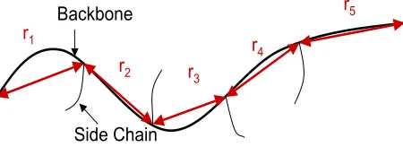
Figure 4: Distance r between cluster interaction points for a single Nafion polymer chain.

in-plane PTFE bond angle in this case is a simplifying assumption.

When a bond placement would locate the next bond within a cluster, another random number is generated to find an alternate but viable low energy conformation. If all out-of-plane rotation angles result in cluster coincidence, the chain is terminated. When a bond corresponding to a pendant chain connection point is being placed, of the possible±15oand±120oout-of-plane PTFE rotations, the angle that minimizes the distance between the carbon atom with the attached side chain and the nearest cluster is used. It is assumed that the pendant chain terminal ionic group successfully communicates with the nearest cluster if the distance between the backbone connection point and the nearest cluster is within 8 ˚A. This value is an estimate of the fully extended length of the pendant chain. It is found that application of this value leads to between 75% and 92% successful cluster communication depending on the assumed cluster configuration. It is not expected that 100% of the ionic groups will reside within a cluster and thus, this range is deemed reasonable.

Each simulated Nafion backbone chain can have multiple r values as illustrated in Figure 4. Furthermore, the first and last r value for each chain, or free ends, do not support any load, and therefore do not contribute to stiffness. Predictions with and without correction of the free-end effects are considered.

In order to assure statistical validity, a large number of r values (about 10,000) are generated. From this, an expression for the chain length probability density functionP(r) must be estimated. Development of an appropriate expression is the subject of Section 3.

2.2. Macroscopic Model for Estimating Stiffness

number of conformations available for a given state [25],

S(r) =c+klnP(r) (4)

where k is Boltzmann’s constant and c is a constant of integration which drops out when the difference in entropy for the unperturbed configuration is taken with respect to the distorted con-figuration. In this approach it is assumed that under load the rotation about the individual bonds is unrestricted which allows the assumption that the Helmholz free energy is strictly a function of entropy. For the assumptions of rubberlike elasticity, the “three chain” model, as described by Treloar [32], yields the relation

∆S= ν 3

h

S(roα) + 2S(roα−1/2)−3S(ro) i

, (5)

for the change in entropy upon distortion. Hereν is the number density of network chains,ro is the

root mean square of the r values applied in the development ofP(r), andα =L/Li is the relative length of the sample. The nominal stressf∗ _{is then given by}

f∗_=−T

∂∆S ∂α

T

=₋νkT ro 3

h G′_(r

oα)−α−3/2G′(roα−1/2) i

(6)

whereG(r) = lnP(r) and G′_{(r) =} dG(r)

dr . The corresponding modulus [f∗] is given as

[f∗_{] =} f∗

α₋α−2. (7)

For small strains (α→1), the modulus in (7) approaches Young’s modulus for the polymer matrix alone; this small strain modulus will be referred to as Einit. The global Youngs’s modulus, Eave, is expected to be lower than Einit due to the volume fraction of hydrophilic clusters which are not expected to be load bearing. Because only the global stiffness,Eave, is experimentally available the means to properly expressEinit, and subsequently relate it toEave are required. Consider first the

Substituting equation (6) into equation (7) and applying L’Hˆopital’s rule, yields the relation

Einit=−νkT ro

6

(

roP(ro)P′′(ro)−ro[P′(ro)]2+P(ro)P′(ro)

[P(ro)]2

)

(8)

for the initial stiffness.

In order to relateEinittoEave, it is first noted thatEinitis directly analogous to matrix stiffness, Em, of classic composite materials theory. Thus, a modified Voigt-Reuss approximation for plane stress [34] is used to relateEinit to the experimentally available values, Eave. This approximation

is given by

Einit =Em = 1_f Eave=VpEave (9)

wheref is the volume fraction not taken up by water, which can be equivalently expressed in terms of the normalized volume after uptakeVp (i.e., if upon hydration the volume increases by 44%, then

Vp is 1.44).

Traditionally RIS has been used for the purpose of studying mechanical response trends where model predictions described by equations (6) and (7) are normalized with respect tovkT. However, a value must be assigned to this parameter in order to predict stiffness. Identification of the number density of chains ν requires the application of some simplifying assumptions. To begin, ν is given by

ν= ρNA

MWc−c

(10)

whereρ is the material density,NA is Avagadro’s number, and MWc−c is the molecular weight of

the portion of the chain between two cluster communication points.

The material density is a readily available, experimentally determined value, whereas Avagadro’s number is a constant. This leaves MWc−c, which is estimated based on the percentage of successful

cluster communications are sufficiently infrequent that it is highly improbable that there would be two failures in sequence. Thus, a single failure corresponds to a local MWc−c of 1562 g/mol.

Applying these values as a ratio of their occurrence is then used to estimate MWc−c. For example,

if the failure rate is 15%, then MWc−c≈0.85(781) + 0.15(1562) = 898 g/mol.

3. Statistical Analysis

The details of the statistical fitting methods applied to the development of variousP(r) expressions for the same distribution ofr values are discussed in [31]. Provided here is a brief overview of the cubic spline and Johnson family methods. In the traditional approach of RIS Monte Carlo theory, a cubic spline approach is used to estimate P(r). The simulation-generated r values are divided into groups, or bins, and a knot value is specified for each bin so that on each interval (delimited by the knots), a cubic polynomial is fit to the data. If we define the indicator function Li(r) for the subinterval (ki, ki+1], where ki is the ith knot, as

Li(r) =

  

 

1, forki < r≤ki+1,

0, otherwise,

(11)

then the result is a piecewise-polynomial estimate of P(r) of the form

P(r) = 1

K

n∗ X

i=1

Li(r)Ai(r−ki)3+Bi(r−ki)2+Ci(r−ki) +Di, (12)

where n∗ _{is the number of knots, A, B, C, and D are the corresponding coefficients of the cubic}

where the number and location of knots is varied, in order to illustrate the physical implications of using a cubic spline approach.

Alternatively, the application of the Johnson family of distributions for density estimation is clearly defined, effectively eliminating any ambiguity in defining the fitting procedure. Further, unlike the coefficients in the cubic spline approach, the various parameters of the Johnson distribu-tion have specific statistical meaning. Lastly, the Johnson distribudistribu-tion only requires the estimadistribu-tion of four parameters and the resulting expression can be easily applied in equations (4)–(8).

In general, the probability density function P(r) based on the Johnson distributions has the form

P(r) = δ

λ√2πf ′

r−ξ

λ

exp

−1₂

h

γ+δfr−ξ λ

i2

, (13)

whereδand γ are shape parameters,λis a scale parameter,ξ is a location parameter, the function

f(_·) is defined according to the applied distribution family, andf′_{(·) is the first derivative of f(·)}

with respect tor [31, 35]. The distribution families definingf(·),f′_{(·), andf}′′_{(·) are}

f(y) =

                

ln(y), for the SL (lognormal) family, ln(y+py2_{+ 1), for the S}

U (unbounded) family, ln(₁₋y_y), for the SB (bounded) family,

y, for the SN (normal) family;

(14)

f′_(y)≡ df(y)

dy =                 

1/y, for theSL (lognormal) family andy >0, 1p

y2_{+ 1, for theS}

U (unbounded) family and all real y, 1/[y(1−y)], for theSB (bounded) family and y∈(0,1),

1, for theSN (normal) family and all real y;

f′′_(y)≡ d 2_f(y)

dy2 =                  −1

y2_{, for theS}

L family and y >0,

−y

(y2+ 1)3/2, for theSU family and all real y,

−(1−2y)

[y(1−y)]2, for theSB family and y∈(0,1), 0, for theSN family and all realy.

(16)

The bounds on these distributions are

H=                 

[ξ,+∞) for the SL (lognormal) family, (−∞,+∞) for the SU (unbounded) family, [ξ, ξ+λ] for the SB (bounded) family, (−∞,+∞) for the SN (normal) family.

(17)

Using equations (13)–(17), the functionG(r) can be written as

G′_{(r) =} f ′′r−ξ

λ

−δhf′r−ξ λ

i2h

γ+δfr−ξ λ

i

λf′

r−ξ λ

. (18)

When this expression is substituted into equation (7), the resulting stiffness expression as a function of distortion is given by

[f∗_{] =−} roνkT

3(α₋α−2₎   

 

f′′roα−ξ

λ

−δhf′roα₋ξ

λ

i2h

γ+δfroα₋ξ

λ

i

λf′

roα₋ξ

λ

−α−3/2

f′′roα−1/2₋ξ

λ

−δhf′roα−1/2₋ξ

λ

i2h

γ+δfroα−1/2₋ξ

λ

i

λf′roα−1/2₋ξ

λ      . (19)

4. Predictions and Discussion

While a total of 135 to 225 repeat units (Figure 2) per ionomer chain is identified as the target, the chain length is typically terminated much earlier due to chain collision with a cluster. Actual simulated chain lengthsmnever exceeded 45. While early termination clearly leads to non-physical predictions of total chain length, it is not believed that this early termination presents a significant problem in the development of an appropriate P(r) expression because it is the lengths between cluster interactions which dictate the elastic properties of the material. To ensure this, analyses have been performed where all chain lengths are included (including those which terminated early) as well as for the more physical case where all initial and final lengths are discarded to eliminate end-effects. Thus, in the current study, correction of free-end effects not only addresses the reality that free ends do not contribute to material stiffness, but also necessarily eliminates early termination effects. (For discussion of free end effects, see for instance, Treloar [22].)

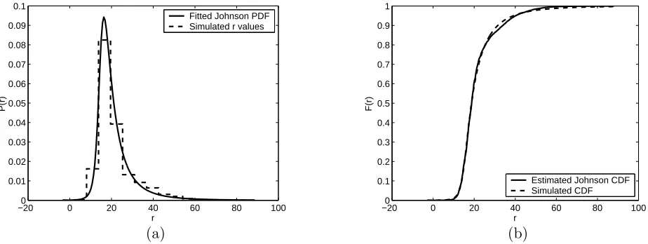
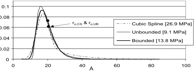
Figures 5 and 6 demonstrate the effect of deleting the first and lastr value for each chain. From these two figures, it is evident that removing the end effects for each simulated backbone chain greatly improves the behavior of the data in the lower tail. Those r values computed from chains with only one or two bonds have been eliminated and, as a result, the second mode in the lower tail of the density in Figure 5 is not as prominent in the density shown in Figure 6. Consequently, correction of free-end effects has the added advantage of greatly improving the accuracy of the Johnson fit since in general the Johnson distribution is not sufficiently flexible to quantify bimodal behavior.

5. Predicted Stiffness Values

Applying Equation (9), the matrix stiffness (Einit = Em) is estimated to be 120 MPa and 115 MPa for Li+ and Na+, respectively, where these values are based on the experimentally measured stiffness values (Eave) of 75 MPa and 80 MPa for the Li+and Na+cases [8]. Figures 7–14 illustrate the predicted probability density functions, with the location ofro indicated; corresponding stiffness

−200 0 20 40 60 80 100 0.01 0.02 0.03 0.04 0.05 0.06 0.07 r P(r)

Estimated Johnson PDF Simulated PDF

−200 0 20 40 60 80 100

0.1 0.2 0.3 0.4 0.5 0.6 0.7 0.8 0.9 1 r F(r) Simulated CDF Estimated Johnson CDF

(a) (b)

Figure 5: Estimated PDF (a) and CDF (b) for the sodium/rectangular case using a Johnson unbounded density function.

−200 0 20 40 60 80 100

0.01 0.02 0.03 0.04 0.05 0.06 0.07 0.08 0.09 0.1 r P(r)

Fitted Johnson PDF Simulated r values

−200 0 20 40 60 80 100

0.1 0.2 0.3 0.4 0.5 0.6 0.7 0.8 0.9 1 r F(r)

Estimated Johnson CDF Simulated CDF

(a) (b)

Figure 6: Estimated PDF (a) and CDF (b) for the sodium/rectangular case using a Johnson unbounded density function with corrected end effects.

short chain lengths. Per the discussion of the previous section, there is no physical reason, other than uncorrected end-effects, to justify the existence of this second mode as reasonable. Therefore, because of the aforementioned difficulties associated with fitting the cubic spline case even to reliable distribution data, no further cubic spline fits were employed for the nonphysical cases (uncorrected end-effects).

Because we expect all considered cases to have similar predicted stiffness values (120 MPa and 115 MPa for Li+ _{and Na}+ _{respectively), the bounded Johnson distribution is deemed favorable.}

Table 2: Initial stiffness predictions [MPa] per statistical methodology, end effects neglected. Cation/Grid Orientation Cubic Spline Johnson Unbounded Johnson Bounded

Sodium, Cubic 3.5 3.2 6.4

Sodium, HCP 3.4 9.8

Lithium, Cubic -1.0 10.4

Lithium, HCP 37.8 9.5

Table 3: Initial stiffness predictions [MPa] per statistical methodology, corrected end effects. Cation/Grid Orientation Cubic Spline Johnson Unbounded Johnson Bounded

Sodium, Cubic -6.6 1.0 9.8

Sodium, HCP 26.9 9.1 13.8

Lithium, Cubic 27.8 4.0 13.6

Lithium, HCP 25.6 18.1 18.3

range (standard deviation of 3.6 MPa from the mean of 10.0 MPa), while the others have much more scatter (standard deviation of 12.9 MPa from the mean of 3.7 MPa for the Johnson unbounded case and standard deviation of 15.9 MPa from the mean of 25.6 MPa for the cubic spline case); (b) the previously noted trend for sodium being marginally softer than lithium is most closely observed in the Johnson bounded case; and (c) the Johnson bounded yielded no negative stiffness predictions.

0 0.02 0.04 0.06 0.08 0.1

0 20 40 60 80 100

Cubic Spline[3.5 MPa] Unbounded [3.2 MPa] Bounded [6.4 MPa]

Å

Figure 7: Na+ Cubic Configuration with neglected end effects. PDF curves for the distribution of r-values and corresponding root mean square value,ro, for cubic spline, Johnson bounded, and

Johnson unbounded distributions.

0 0.02 0.04 0.06 0.08 0.1

0 20 40 60 80 100

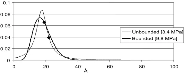
Unbounded [3.4 MPa] Bounded [9.8 MPa]

Å

Figure 8: Na+_{HCP Configuration with neglected end effects. PDF curves for the distribution ofr}

-values and corresponding root mean square value,ro, for Johnson bounded and Johnson unbounded distributions.

Å

0 0.02 0.04 0.06 0.08 0.1

0 20 40 60 80 100

Unbounded [-1.0 MPa] Bounded [10.4 MPa]

Figure 9: Li+Cubic Configuration with neglected end effects. PDF curves for the distribution ofr -values and corresponding root mean square value,ro, for Johnson bounded and Johnson unbounded

Å

0 0.02 0.04 0.06 0.08 0.1

0 20 40 60 80 100

Å

Unbounded [37.8 MPa]

Bounded [9.5 MPa]

Figure 10: Li+HCP Configuration with neglected end effects. PDF curves for the distribution ofr -values and corresponding root mean square value,ro, for Johnson bounded and Johnson unbounded

distributions.

-0.02 0 0.02 0.04 0.06 0.08 0.1

0 20 40 60 80 100

Cubic Spline[-6.6 MPa]

Unbounded [1.0 MPa]

Bounded [9.8 MPa]

Å

Figure 11: Na+ Cubic Configuration with corrected end effects. PDF curves for the distribution of r-values and corresponding root mean square value,ro, for cubic spline, Johnson bounded, and

Johnson unbounded distribution.

0 0.02 0.04 0.06 0.08 0.1

0 20 40 60 80 100

Cubic Spline[26.9 MPa]

Unbounded [9.1 MPa]

Bounded [13.8 MPa]

Å

ro,CS& ro,UB

Figure 12: Na+ _{HCP Configuration with corrected end effects. PDF curves for the distribution}

Å 0

0.02 0.04 0.06 0.08 0.1

0 20 40 60 80 100

Cubic Spline[27.8 MPa]

Unbounded [4.0 MPa]

Bounded [13.6 MPa]

Å

Figure 13: Li+ Cubic Configuration with corrected end effects. PDF curves for the distribution of r-values and corresponding root mean square value,ro, for cubic spline, Johnson bounded, and

Johnson unbounded distributions.

Å 0

0.02 0.04 0.06 0.08 0.1

0 20 40 60 80 100

Cubic Spline[25.6 MPa]

Unbounded [18.1 MPa]

Bounded [18.3 MPa]

Å ro,CS

ro,UB& ro,Bo

Figure 14: Li+ HCP Configuration with corrected end effects. PDF curves for the distribution of

r-values and corresponding root mean square value, ro, for cubic spline, Johnson bounded, and

Johnson unbounded distributions.

Å

-0.02 0 0.02 0.04 0.06 0.08 0.1

0 20 40 60 80 100

10 Knots [-2.6 MPa] (last knot length reduced) 10 Knots [-3.8 MPa] (1 knot removed from tail) 11 Knots [-6.6 MPa] All ro

Region Varied

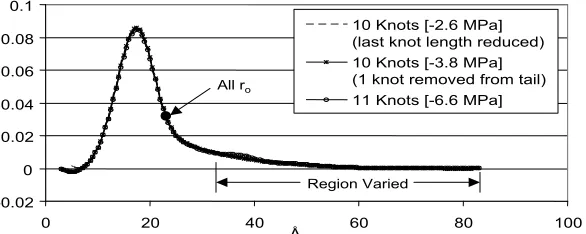
Figure 15: Na+ Cubic Configuration with corrected end effects. PDF curves for the distribution of r-values and corresponding root mean square value, ro, for minor variations in cubic spline

The traditional cubic spline approach is deemed the most unreliable of the considered methods because of the ill-defined methodology for fixing the knots. Any perception of consistency in stiffness predictions (based on the last 3 entries for cubic spline approach in Table 3), is somewhat misguided as these results are to some degree ‘manufactured’ by moving the knots until an appropriate response is predicted. While this may be acceptable for well-studied cases, one of the primary goals of modeling is to predict those cases which are not easily studied experimentally. As demonstrated in Figure 15, by altering the placement and number of knots we were able to alter the predicted stiffness. In the illustrative example of 15, the cubic spline approach not only yields non-physical predictions (negative stiffness) from a data set for which the Johnson distributions yield positive predictions, but also illustrates that minor variation to the number and placement of knots has non-negligible impact on predicted stiffness. The single greatest challenge with cubic spline is discerning the level of detail which is physically appropriate. With the Johnson cases, no qualitative judgment of this sort is required.

It is proposed that the reason the Johnson bounded case offers the most stable predictions is because thero position is consistently nearer the peak of the distribution. At this point in theP(r)

curve, the expression

roP(ro)P′′(ro)−ro

P′_(r

o)2+P(ro)P′(ro)<0, (20)

which is a necessary condition for reasonable stiffness predictions (based on Equation (8)), is more likely to be satisfied becauseP′′ _{is more likely to be negative (while we are generally assured that} P >0 and P′ _{<0). Further, the magnitude of P}′ _{is likely less sensitive to small changes in r}

o in

this region.

6. Predicted Stress-Strain Responses

(B) Na+_{Normalized Stress vs. Strain}

0.00 0.05 0.10 0.15

0 0.05 0.1 0.15 0.2

strain

f*

/Ein

it Experimental

Cubic Config. HCP Config.

(A) Li+ _{Normalized Stress vs. Strain}

0.00 0.05 0.10 0.15 0.20 0.25

0 0.05 0.1 0.15 0.2 0.25 0.3 0.35 0.4

strain

f*

/Ein

it Experimental

Cubic Config.

HCP Config.

Figure 16: Normalized Stress-Strain behavior of experimental data [29] and model, both Cubic and HCP cluster configurations, with Corrected End Effects.

on the Johnson bounded with corrected end effects cases, it can be shown that within the range of several percent strain, all of the Johnson predictions (normalized with respect toEinit) yield similar stress-strain response trends. The cubic spline cases introduce considerably more variability and, in general, yield normalized stress predictions that are considerably higher than the Johnson cases at a given strain.

Further, it is not appropriate to compare model and experiment predictions beyond several percent strain because beyond this point the strain response is known to be effected by the hydration technique. Therefore, within the context of the traditional use of RIS (viz., normalized comparisons only), the modeling methodology is deemed appropriate and useful for study of solvated Nafion, both in terms of treatment of cluster communication concept for identification of load bearing chain lengths and the statistical analysis.

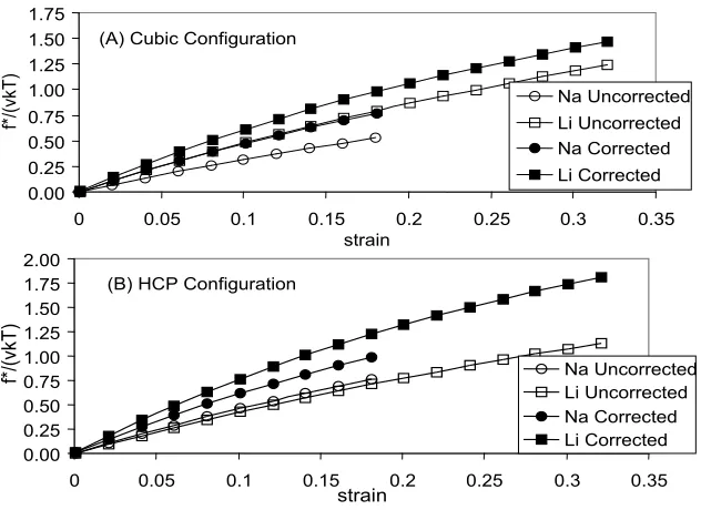
(B) HCP Configuration 0.00 0.25 0.50 0.75 1.00 1.25 1.50 1.75 2.00

0 0.05 0.1 0.15 0.2 0.25 0.3 0.35 strain f* /( vkT ) Na Uncorrected Li Uncorrected Na Corrected Li Corrected (A) Cubic Configuration

0.00 0.25 0.50 0.75 1.00 1.25 1.50 1.75

0 0.05 0.1 0.15 0.2 0.25 0.3 0.35 strain f* /( vk T ) Na Uncorrected Li Uncorrected Na Corrected Li Corrected

Figure 17: Stress normalized with respect to νkT versus strain for bounded distributions, with neglected and corrected end effects.

0.00 0.25 0.50 0.75 1.00 1.25 1.50 1.75 2.00

0 0.05 0.1 0.15 0.2 0.25 0.3 0.35

strain f* /( vkT ) Na Cubic Li Cubic Na HCP Li HCP

Figure 18: Stress normalized with respect toνkT versus strain, corrected end effects with bounded distributions, for Cubic and HCP configurations.

cluster diameter and volume fractions are held constant for the two cases, it must be concluded that cluster morphology plays an important role in material stiffness.

(B) (vkT) Normalized

-0.80 -0.60 -0.40 -0.20 0.00

0.00 0.05 0.10 0.15 0.20 0.25 strain

f*

/(

vk

T

) -6.6 MPa

-3.8 MPa -2.6 MPa (A) EiNormalized

0.00 0.25 0.50 0.75 1.00 1.25

0.00 0.05 0.10 0.15 0.20 0.25 strain

f*

/Ei

-6.6 MPa -3.8 MPa -2.6 MPa

Figure 19: Na+Cubic configuration with corrected end effects. Stress-strain predictions normalized with respect toEi and vkT for minor variations in cubic spline distributions (refer to Figure 15).

Figure 19 revisits the cubic spline cases of Figure 14 to illustrate the corresponding predicted stress-strain response trends. Recalling from Figure 15 that subtle changes toP(r) via knot selection lead to non-negligible variation in the stiffness predictions, it is observed that the same continues to be true for stress-strain response trends. In particular, the variations in response illustrated in Figure 19, where the predictions are normalized with respect to νkT, is significant as this normalization has often been used to infer physical meanings between similar distribution data (i.e., increasing volume fractions of rigid inclusions [26]). It is of course presumed that previous practitioners of this modeling methodology have been aware of this sensitivity when present in their own systems and were thus potentially subjected to a substantial task in identifying the proper cubic spline fit. It is thus again emphasized that application of the Johnson bounded case represents both stability and simplification in RIS predictions as compared to the cubic spline case.

7. Johnson Parameter Perturbation Results

the most significant impact; variation ofδ (shape/peak parameter) andλ(scale/spread parameter) have weaker but discernable effects; and variation ofγ (shape/skewness parameter) has a variable effect.

Table 4: Perturbation study of Lithium, HCP, Johnson Bounded, corrected end effects.

ξ δ λ γ ro (˚A) Ei (MPa) 4.17 2.977 248.7 8.689 18.055 16.4 5.17 2.977 248.7 8.689 19.0275 18.1 6.17 2.977 248.7 8.689 20.0027 21.1 5.17 2.777 248.7 8.689 16.6582 17.0 5.17 2.977 248.7 8.689 19.0275 18.1 5.17 3.177 248.7 8.689 21.4726 19.6 5.17 2.977 244.7 8.689 18.8024 18.3 5.17 2.977 248.7 8.689 19.0275 18.1 5.17 2.977 252.7 8.689 19.2525 18.0 5.17 2.977 248.7 7.689 24.1299 16.4 5.17 2.977 248.7 8.689 19.0275 18.1 5.17 2.977 248.7 9.689 15.2235 19.9

Increasing ξ always leads to an increase in the predicted stiffness. To interpret the physical significance of this, the analysis must be considered within the context of Equation (19). From this equation it is seen that the chain densityν is held constant while effectively increasing the typical chain length. In order for this to happen both the material density ρ and molecular weight must rise, meaning that any given bond within the higher ξ material is carrying less load for a given external load. This corresponds to an increase in the load carrying capability for the bulk material, or higher stiffness.

8. Conclusions

A new multiscale modeling technique for the prediction of ionomer stiffness has been presented through extension of traditional RIS theory. Prediction stability is introduced by fitting the chain length distributionP(r) using a Johnson bounded distribution rather than the commonly applied cubic spline approach. For all considered cases, the Johnson bounded cases yielded the most stable stiffness and stress-strain predictions, and the cubic spline approach yielded the most unreliable (variable) results. A Johnson distribution is further preferred because its parameters can be related to physical characteristics in the polymer, whereas cubic spline parameters cannot. Further, the normalized stress-strain response measured experimentally is consistent with that predicted by the model up to several percent strain (when appropriately normalized). Direct prediction of stiffness and stress-strain response may ultimately be possible once sources of error such as early termination and estimation of the molecular weight are addressed in detail. Lastly, the current model gives insight into significant material parameters. For example, correction of end effects yields higher predicted stiffness; thus end effects are non-negligible in this relatively short chained system. Further, the stiffness predictions are sensitive to the assumed cluster morphology, offering a tool for studying this unresolved physical issue.

Acknowledgements

References

[1] K. Sadeghipour, R. Salomon, and S. Neogi: Development of a novel electrochemically active membrane and ’smart’ material based vibration sensor/damper.Smart Mater. Struc.1(2), 172 (1992).

[2] K. Oguro, Y. Kawami, and H. Takenaka: An actuator element of polyelectrolyte gel membrane-electrode composite.Osaka Kogyo Gijutsu Shikensho Kiho 43(1), 21 (1992).

[3] Yoshito Osada and Mariko Hasebe: Electrically Activated Mechanochemical Devices Using Polyelectrolyte Gels. Chem. Lett.1285 (1985).

[4] Masahiro Irie: Photoresponsive Polymers. Reversible Bending of Rod-Shaped Acrylamide Gels in an Electric Field.Macromolecules 19, 2890 (1986).

[5] Tohru Shiga and Toshio Kurauchi: Deformation of Polyelectrolyte Gels Under the Influence of Electric Filed.Journal of Applied Polymer Science 39(11/12), 2305 (1990).

[6] M. Shahinpoor: Conceptual Design, Kinematics and Dynamics of Swimming Robotic Struc-tures Using Ionic Polymeric Gel Muscles.Smart Materials and Structures 1(1), 91 (1992).

[7] M. Shahinpoor, Y Bar-Cohen, J.O. Simpson, and J. Smith: Ionic polymer-metal composites (IPMCs) as biomimetic sensors, actuators and artificial muscles - a review. Smart Mater. Struct.7(6), R15 (1998).

[8] Y. Bar-Cohen (Editor), Electroactive Polymer (EAP) Actuators as Artificial Muscles - Re-ality, Potential, and Challenges (SPIE- The International Society for Optical Engineering, Bellingham, Washington, 2001).

[9] M. Mojarrad and M. Shahinpoor: Ion exchange membrane-platinum composites as electrically controllable artificial muscles.SPIE Proc 2779 p. 1012 (1996).

[10] S. Nemat-Nasser: Micromechanics of Actuation of Ionic Polymer-metal Composites (IPMCs).

J. Appl. Phys.92(5), 2899 (2002).

[11] K. Farinholt, K. Newbury, M. Bennet, and D. Leo: An Investigation into the Relationship between Charge and Strain in Ionic Polymer Sensors, inFirst World Congress on Biomimetics

and Artificial Muscles (Albuquerque, NM, 9 -11 December 2002).

Macromolecules 15, 101 (1982).

[13] V. K. Datye, P.L. Taylor, and A. J. Hopfinger: Simple Model for Clustering and Ionic Transport in Ionomer Membranes.Macromolecules 17, 1704 (1984).

[14] V. K. Datye and P. L. Taylor: Electrostatic Contributions to the Free Energy of Clustering of an Ionomer.Macromolecules 18, 1479 (1985).

[15] A. Lehmani, S. Durand-Vidal, and P. Turq: Surface Morphology of Nafion 117 Membrane by Tapping Mode Atomic Force Microscope.J. Appl. Poly. Sci. 68, 503 (1998).

[16] V. Barbi, S. Funari, R. Gehrke, N. Scharnagl, and N. Stribeck: Nanostructure of Nafion membrane material as a function of mechanical load studied by SAXS. Polymer 44, 4853 (2003).

[17] P.G. de Gennes, Ko Okumura, M. Shahinpoor, and K.J. Kim: Mechanoelectric Effects in Ionic Gels.Europhysics Letters 50(4), 513 (2000).

[18] K. Asaka and K. Oguro: Bending of polyelectrolyte membrane platinum composites by electric stimuli.J. Elec. Chem. 480, 186 (2000).

[19] J. Y. Li and S. Nemat Nasser: Micromechanical analysis of ionic clustering in Nafion perfluo-rinated membrane.Mech. Mater. 32, 303 (2000).

[20] S. Nemat-Nasser and J.Y. Li: Electromechanical response of ionic polymer-metal composites.

J. Appl. Phys.87(7), 3321 (2000).

[21] L.M. Weiland and D.J. Leo: Computational Analysis of Ionic Polymer Cluster Energetics.J.

Appl. Phys.97, 013541 (2004).

[22] L.R.G. Treloar, The Physics of Rubber Elasticity, 3rd ed. (Clarendon Press, Oxford, England, 1975).

[23] W.G.F. Grot, C.E. Munn, P.N. Walmsley, in 141st Meeting of the Electrochemical Society, Houston, TX, May 1972.

[24] P.J. Flory, Statistical Mechanics of Chain Molecules (Hanser Publishers, New York, New York, 1988).

Polydimethyl-siloxane short-chain unimodal networks.J. Chem. Phys. 79(11), 5705 (1983).

[26] Q.W. Yuan, A. Kloczkowski, J.E. Mark, and M.A. Sharaf: Simulations on the Reinforcement of Poly(dimethylsiloxane) Elastomers by Randomly Distributed Filler Particles. J. Poly. Sci

B: Poly. Phys 34, 1647 (1996).

[27] M.A. Sharaf, A.Kloczkowski, and J.E. Mark: Monte Carlo simulations on reinforcement of an elastomer by oriented prolate particles.Comp. Theo. Poly. Sci.11, 251 (2001).

[28] M.A. Sharaf, R.H. Abouhussein: Computer Simulations on the chain deformations of Poly(Ethylene) by Randomly-Oriented Prolate Filler particles Arranged on a Cubic Lattice.

Poly. Preprints 44(1), 1258 (2003).

[29] M.A. Sharaf, I.M. Jasiuk, K.I. Jacob: Monte Carlo Simulations combined with Micromechanics to predict effective elastic moduli of elastomeric nanocomposites filled with unidirectional rigid inclusions.Poly. Preprints 44(1), 1249 (2003).

[30] T.W. Bates and W.H. Stockmayer: Conformational Energies of Perflouroalkanes. II Dipole Moments of H(CF2)nH.Macromolecules 1(1), 12 (1968).

[31] J.L. Mathews, E.K. Lada, L.M. Weiland, R.C. Smith, D.J. Leo: Monte Carlo Simulation of a Solvated Ionic Polymer with Cluster Morphology. Submitted toSmart Materials and Structures

January 2005.

[32] K.A. Page and R.B. Moore: Correlations between bulk mechanical relaxations and spin dif-fusion times in Perfluorosulfonate Ionomers: Molecular Origins of Mechanical Relaxations.

Polymer Preprints 44(1), 1144 (2003).

[33] A.K. Phillips and R.B. Moore: Phase Behavior in Solution Processed Perfluorosulfonate Ionomers.Polymer Preprints 44(1), 1142 (2003).

[34] R.M. Jones, Mechanics of Composite Materials (McGraw-Hill Book Company, New York, New York, 1975).

[35] D.J. DeBrota, R.S. Dittus, S.D. Roberts, J.R. Wilson, J.J. Swain, and S. Venkatraman: Mod-eling Input Processes with Johnson Distributions.Proc. of the Winter Simulation Conf.p. 308 (Piscataway, New Jersey: IEEE, 1989).