Analysis of multiple capture-recapture data using band-recovery methods

Key

UJords:

ANALYSIS OF MULTIPLE CAPTURE-RECAPTURE

DATA USING BAND-RECOVERY METHODS

CAVELL BROWNIE and KENNETH H. POLLOCK

Department of Statistics

North Carolina State University

Box 8203, Raleigh, NC 27695-8203 USA

Institute of Statistics

Mimeograph Series No. 1647

North Carolina State University

Raleigh, North Carolina

October, 1984

Capture-recapture models; band return models; fossil data;

SUMMARY

One simple approach to the analysis of multiple capture-recapture

data is to use only first and last captures and carry out the band-recovery

analyses of Brownie et

aZ.

(1978). In this paper, we present the loss in

efficiency of this approach compared to the Jolly-Seber analysis and its

age-dependent extension. We also develop estimates of capture probabilities

and population sizes for the first and last capture data. Finally, we

present an example from the fossil record where only first and last capture

data are available, so that the Jolly-Seber model cannot be used.

1.

Introduction

Procedures for the statistical analysis of band or tag return data which

are described in a handbook by Brownie et

aZ.

(1978) are now being widely

used by wildlife and fisheries biologists. This is due in part to the

availability of supporting computer software from the U. S. Fish and

Wildlife Servi~e, Patuxent Wildlife Research Center, Laurel, Maryland.

Brownie et

aZ.

(1978) suggest that until analogous methodology

involving a comparable series of models is developed for live or multiple

recapture data, "there is always the possibility of analyzing live

recapture data by dead-recovery formulae." This is accomplished by

ignoring all but the first and last capture occasions for each animal

(Brownie et

aZ.,

1978, p. 175).

One objective of this paper is to emphasize that this approach (e.g.,

Mardekian and McDonald, 1981) is now outdated. The appropriate methodology

for multiple capture-recapture data has now been developed by Pollock (1981),

computer programs are now available. Jolly-Seber analyses (Jolly, 1965;

Seber, 1965) can be performed using "POPAN" developed by Arnason and

Baniuk (1978) or a program available from J. E. Hines and J. D. Nichols,

U. S. Fish and Wildlife Service, Patuxent Wildlife Research Center, Laurel,

Maryland 20811. Hines and Nichols also have a program to carry out the

analysis for the age-dependent version of the Jolly-Seber model.

Biologists should be made aware that use of the band-recovery models with

live recapture data involves "throwing away" data, with consequent loss

of efficiency. We show that the loss in efficiency for survival estimators

can be substantial.

Recently, Nichols and Pollock (1983) and Conroy and Nichols (1984)

have shown that capture-recapture and band-recovery methodology can be

used in the analysis of fossil data. In that context, there are some data

sets where only first and last capture information is available. Therefore,

a second objective of this paper is to present new estimators and their

standard errors, of capture probabilities and population sizes which will

be useful to paleobiologists. We also show their loss in efficiency if

complete history information were available. An example using real fossil

data is presented, and finally, a general discussion is presented.

2.

Experimental Situation

The situation considered is a capture-recapture study, described for

example by Jolly (1965), Seber (1965), or Pollock (1981), involving

in efficiency incurred by discarding intervening capture records and

applying band-recovery analyses (e.g., Models 1 and H

l in Brownie et aZ.,

1978) to the first and last captures only. The single age class

situation (cf. Jolly, 1965; Seber, 1965) is considered first, and then

two age classes (cf. Pollock, 1981).

For simplicity, it is assumed that there are no losses on capture.

Otherwise, the usual assumptions are made that animals suffer independent

fates, and that the population is homogeneous, at least within an

age class, to time-specific survival and capture probabilities (see for

example, Seber, 1982, p. 196).

3.

One age Class

3.1 Notation

Notation used is, in general, consistent with that in Chapter 5 of Seber

(1982). However, comparison between the multiple capture-recapture and

band-recovery methods makes it necessary to extend this Dotation and

achieve some compromise with that in Brownie et aZ. (1978).

For the single age class Jolly-Seber model described by Seber (1982,

S is the number of sampling occasions.

N. is the total number in the population just before the ith

I

sample, i=l, ...,s.

M. is the number of marked animals in the population before the

I

ith sample, j=l, ...,s, M

1=O.

U.

I

<p.

I

Pi

=

1-q.I

= N.-M. , i=l, .•. ,s. I I

is the survival rate from i to i+1, i=l, ... ,s-l.

is the probability an animal is captured in the ith sample

given that it is present, i=2, •..,s.

U. is the number first caught in the ith sample, i=1, ••.

,s-1-I

m. is the number of marked animals caught in the ith sample,

I

i=2, ...,s.

R. is the number of marked animals released after the ith sample,

I

i=l, ••.,s-l . (R.

=

u.+m. assuming no losses on capture).

I I I

r. is the number of the R. that are captured at least once after

I I

the ith sample, i=l, ... ,s-l.

z. is the number captured before and after, but not in, the ith

I

sample, i=2, ..• ,s-1.

X. is the probability an animal present just after the ith sample

I

is not captured again, and is represented recursively by

i-X· =

I

Nichols, 1984).

In order to apply the band-recovery Model 1 analysis to the multiple

recapture data, and obtain valid variance estimates, the recapture data

are used to construct a recovery matrix. The number of new releases after

sample i , u.

,

, and the number of this cohort last captured on each following

sampling occasion are recorded in the ith row and appropriate columns of

the recovery matrix (see, e.g., Mardekian and MacDonald, 1981; Conroy and

*

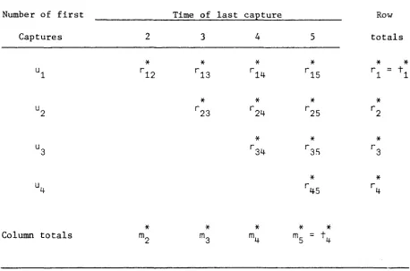
Entries in the recovery matrix are denoted r .. , where

IJ

*

r .. is the number of the u. first captured and released at the ith sample,

IJ I

that are recaptured for the last time in the jth sample, i=l, ... ,s-l,

j=i+l, ...,s (see Table 1).

[Table 1J

As indicated in Table 1, summary statistics based on the recovery

*

matrix {r .. } are

'J

i=l, ... ,s-l

*

m.

,

*

r.

I

*

and t.

I

the number of marked animals recaptured for the last time

in the ith sample, i=2, ...,s.

the number subsequently recaptured of the

u.

first

I

captured in the ith sample, i=l, ... ,s-l ,

the number first captured before or in the ith sample

and subsequently recaptured after the ith sample,

*

*

*

*

* *

(t₁ = r

*

*

*

The relationship between these statistics, m.

,

r.

,

t. and

I I I

C.

,

R.

,

T.

in the usual band-recovery formulation (Brownie

et aZ. ,

I I ' I

1978, p. 13) is not entirely straightforward, because release and

recovery (recapture) in the same period occurs in the typical band-recovery

study but cannot occur in the recapture studies considered here. Thus, the

*

diagonal elements of the usual recovery matrix are missing in {r .. } and

IJ

columns are shifted to the left.

3.2

Estimators and Large SampZe Variances

Estimating survival rates is the main objective in many recapture studies,

and is considered first. As noted by Seber (1982, p. 215), equivalent

results are obtained if survival rate estimators and their large-sample

variances are derived using a likelihood with the u. (new releases at i)

I

as random variables, or a likelihood conditional on fixed u. • This is

I

also true for estimators of capture probabilities. Thus, in comparing

estimators of ~. and p. , for the multiple recapture data results are

I I

drawn from Jolly (1965), Seber (1965) (where the u. are random) and from

I

Brownie and Robson (1983) (u. fixed); and for the first and last captures,

I

analogy is made to the band-recovery methods (Brownie

et aZ.,

1978, u.

I

fixed) .

For the multiple recapture data, the Jolly-Seber estimators and

r.

1

[m.

+ Ri+

1_Zi

+

_1]

<p.

=

I i=1, ... ,s-2 (1)

R.""

1 _m

i+1+z i +1 1+1 rj+₁ I

Var{$. ) = <p2 fE(Mi+l-mi+l)E(Mi+l+Ui+l)

[E(r~+ll

-

E{R~+l)J

I _i

1

_Mf+l

E(M. -m. )

[E(~i)

-

E{~i

lJ}

<p. (l-<p. )

(2)

+ I I + I I

E(M.+u. ) E(M.+u.)

I I I I

COV(~i '~i+l)

= -<Pjif!i+1Qi+l

{E(r~+ll

-

E(R~+1)

}

m. I

i=2, ... ,s-1 (3)

p. =

I m. +R. z.fr. I I I I

*

For the first and last capture data, the likelihood of the r ..

IJ

*

conditional on the u. is obtained by noting that the (r. '+1'.' .,r~ ) are

I I , I IS

mutually independent multinomial vectors characterized by

(4)

*

E( r. .) = u.<p • . . .if!. l P ·X.

IJ I I J- J J i=l, ... ,s-l, j=i+l, ... ,s.

INote that var<p.) in Brownie and Robson, 1983, p. 453, is incorrect.

I

By analogy to P[{R .. }] in Brownie and Robson (1976, p. 307), the

IJ

*

likelihood of {r .. } conditional on the u. is

IJ 1

where

*

P[{r .. } ] =

IJ

s-1 1T i=1

[

*

u.

* ]

r._{I , I}.+1

~

... ,r._IS

*

*

*

m.

t.+

₁-r'+₁

f. I <p. 1 1

I I

*

u. -r.

I 1

X·₁

f._I = ~

P X

'fi-1 i i i=1, ... ,s-1

*

*

*

*

A minimal sufficient statistic is (r

1,···,rS_1'

t

2, ...

,t

s_1),

*

*

*

where r. given u. is Binomial (u., 1-X.), and m. given

t.

1 is

1 I I I 1

1-Binomial _(t.

*

_{l ' <p. 1P.}

x. /

(1-X.») •

1- 1- 1 1 I This leads to the maximum likelihood

~

*

estimators 1-X. = (r./u.)

I I 1

r----...;

<p. 1 P , X.

1- I I

* *

*

=

(m./t.

1)(r. 1

/u .

1)

I 1 - 1 - 1- Using

i=1, ... ,s-2 (5 )

p.

=

1

*

r. I

*

u. -r. I 1

*

m. 1

*

*

t.

1-m. 1- I

The large sample variances and relevant non-zero covariances are

Var(~.)

I

(7)

Var(p. )

I =

p?

i--4-

+

1_*~

+

I E(r. l ) u.-E(r.) I 1 1

*

*

E(t. l-m.) 1- I (8)

The estimators based on first and last captures are denoted ~.

,p.

I I

to distinguish them from the Jolly-Seber estimators ~.

,p ..

I I

The estimator

p.

and its variance do not appear in earlier articles

1

and are included here because of their importance in the context of the

example in Section 5. Also important in this context is estimation of

N. (the population size at i), and we present below the appropriate

I

estimator

N.

and its variance. In deriving N. and VarcN.) , it is

I I 1

*

assumed that u. is Binomial (U.,p.) and t. 1 is Binomial CM. ,1-q.X.)

1 1 I 1- I 1 I

with U. and M. fixed and unknown. Thus, VarCN.) as presented below is

I I I

for fixed N. , and is comparable to Jolly's VCN.IN.) (equation (28),

1 I 1

Jolly, 1965).

*

*

*

u. _{t. 1 u. t. l-m.}

* *

N.

= ~+ I - = -;rI 1- I _{(u. -r. +m. ) i=2, ... ,s-1} (9)

*

1 p. _{l-q-:X. I I I}

1 _{I 1 r. m.}

I I

N2 { 1*

1 1 1 q.

x·

-<1-X· )}

VarCN. ) = +

*

*

+

*

+ 1 I I

(10)

I

I ECrj ) ECu. ) ECt. -m. ) ECm_j ) ECu. - r . +m. )

* *

3.3

Loss

in Efficiency

The loss in efficiency due to using only the first and last captures was

examined by comparing the appropriate asymptotic standard errors (se's),

obtained from the variances in the preceeding section. For ~. and ~.

I I

the variances used include the component of variation due to viewing the

number of marked animals surviving to i+l , of those present at i , as

the outcome of a chance process (cf. Jolly, 1965; Seber, 1965; Brownie

et al., 1978), rather than a fixed quantity (cf. Pollock, 1981). It

seems appropriate to include this component of variation because survival

estimates are often used to make comparisons across locations, times or

conditions, and given the same inherent chance of survival, actual survival

will vary from one occasion to another. For comparing

N.

and

N. ,

I I

variances used were conditional on fixed N. , and therefore reflect

I

sampling variation, but not variation due to viewing N. as a random

I

variable (cf. Section 3.2, Jolly, 1982).

Percent loss in efficiency for ~. was calculated as

I

100[1-se($. )/se(~.)J , and analogously for

p.

and

N. .

For simplicity,

I I I I

the u. were assumed equal (u.=u, i=1, ... ,s-1), loss in efficiency being

I I

independent of u in this situation. Also, in each case considered, a

common value was used for the ¢. and for the p. (¢.=¢, i=1, ... ,s-1, and

1 I I

p.=p, i=2, ... ,s). The cases considered included values of

¢

andp likely

I

to obtain in practice. For example, values between 50 and 65% for annual

survival rates are typical for many banding studies, and the recapture

data in Mardekian and MacDonald (1981) yield estimates p. in the 30 to 40%

~

range, while the example in Pollock (1981) yields p. greater than 80%.

I

For a given set of values of ~ p and 5 , loss in efficiency is

not the same for each ~j' i=1, ...,5-2 (or for each

Pi ' N

_{j ) .} To

summarize results, loss in efficiency was calculated for each ~. and

1

individual values averaged. These averages are presented in Table 2 for

the estimators of survival and capture probabilities and population size.

[Table 2J

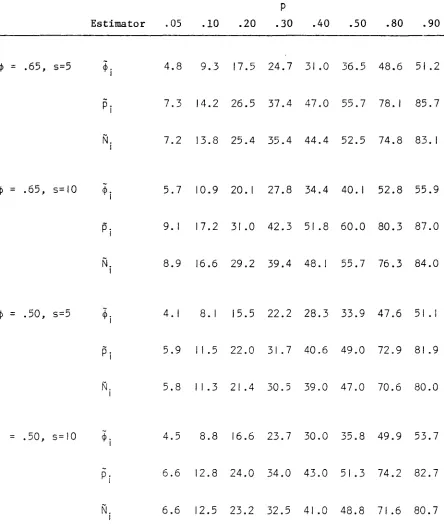
Examination of Table 2 shows that average loss in efficiency is

considerably greater for

p.

and

N.

than for ~.

I 1 1 This seems reasonable,

as intermediate captures have a more direct effect on estimates of

corresponding p. (and hence of N.) than on estimates of survival in

1 1

preceding periods. Loss in efficiency is seen to increase as p increases,

and to a lesser degree, as ~ or the number of capture occasions (hence the

number of intermediate recaptures) increase. Note that for values of

p ~ .30 (corresponding to data in Mardekian and MacDonald, 1981 and

Pollock, 1981), the loss in efficiency is substantial.

In summarizing their results, biologists often report an average

survival rate (e.g.,

1 5-2

;P=-2

I ~.)

5- I

i=l

and a standard error based on

5-3

1

2 I CoV(;P.'~.+l)

. 1 1 I

1=

.,.,.

, as compared to ~ , by

examined the loss in efficiency of ~

5-2

=

-2:-2 1:

~.

5- i=l I

calculating the appropriate standard errors using variance and covariance

formulae in (2) and (7) • For p ~ .3, results were essentially the same as

for cp. in Table 2. For p < _{.8 loss in efficiency tended to be less severe}

r -

,

for the average, <P

,

than for the individual ~. (30 to 40% as compared to

I

40 to 50%). This is because the negative correlation between survival

estimators for adjacent years is smaller in absolute magnitude for the <p. ,

I

-than for the <p.

,

for large p

I

5-2

We also compared asymptotic standard errors for <PH = 1: w.~. and

i=l I I

~H

=

5-2 1:

i=l

v.~.

I I where the weights

w.

I and

v.

I are chosen to minimize the

asymptotic variances of <PH and <PH ' respectively (subject to 1:w_j

=

1 and

1:v_j

=

1). Thus, ~H is the "Hanover estimator" described by Jolly (1982).

This comparison provides information concerning the relative efficiency of

the two maximum likelihood estimators of a constant survival rate, <P ,

obtained assuming constant survival, and (i) applying the Model 2 analysis

of Brownie et al. (1978) to the first and last captures, or (ii) applying

Model B of Jolly (1982) to the complete recapture information (see Appendix

4, Jolly, 1982). Results for loss in efficiency for ~H (relative to ~H)

were very similar to those for ~ (relative to

$)

for all cases considered.

4.

Two age Classes

In this section, we consider estimation of young and adult survival rates

(cp?

and

<P~

respectively) given recapture information recorded separately

I I

for individuals marked as young and as adults. Pollock (1981) provides the

appropriate estimators,

~?

and

~~

, which utilize all the recapture

information. By omitting all but the first and last captures, Model HI

of Brownie

et at.

(1978) could also be used to obtain survival estimates,

-0 -1

~. and ~. , and we are interested in the inefficiency of this latter

I I

procedure.

The relevant estimators and variances are not reproduced here.

~O ~1

However, var(~.) and var(~.) in Pollock (1981) do not allow for a variable

I I

number of survivors at i+1 of the marked animals of appropriate age present

just after sample i . Thus, var(~.)~O and var(~.)~1 of Pollock (1981) were

I I

adjusted (by adding the appropriate Binomial variance) in order to make

-0 -1

comparisons with var(~.) and var(~.) based on the band-recovery Model HI

I I

analysis of first and last captures.

-0 -1

Loss in efficiency for the estimators ~i and ~i is illustrated for

the example in Pollock (1981). For this 4-year study on neck-collared

young and adult giant Canada geese

(Branta canadensis maxima),

the

recapture (i.e., resighting) rates were high (about 90 percent).

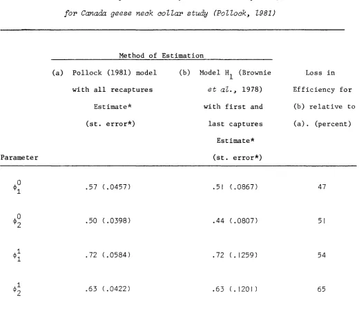
Survival rate estimates and estimated asymptotic standard errors obtained

using the method of Pollock (1981) on all recaptures, and using the

Model HI band-recovery analysis on first and last captures, are presented

in Table 3. No adjustment was made to correct for the neck-collar loss

problem (see Pollock, 1981). The standard errors of ~.~O and ~.~1 in Table 3

I I

are substantially larger than those in Pollock (1981) because here they

include the component of variation due to viewing the numbers of marked

survivors as variables, not fixed quantities.

Loss in efficiency in Table 3 was calculated as in Section 3.3, but

using the estimated standard errors. The roughly 50% loss in efficiency

shows the Model HI analysis to be clearly inferior in terms of precision

of estimates.

5.

Application to Fossil Data

Paleobiologists interested in examination of variation in extinction rates

have made use of compilations of fossil records consisting of the periods

of first and last encounters of the taxa of interest. This "stratigraphic

range data" is analogous to capture-recapture data where records of first

and last capture only are available.

In this setting, individuals correspond to species or taxa and a

sampling occasion corresponds to a geologic period. The first (last)

capture occasion is the earliest (latest) period in which the taxon is

*

encountered in the fossil record, and therefore, r .. is the number of taxa

IJ

first recorded in period i and last encountered in period j. Survival

from the midpoint of one period to the midpoint of the next (~.) is the

I

complement of the extinction rate, the capture probability (p.) is an

I

"encounter probability" or the probability that a taxon is observed in

a period given that it is extant during that period, and the population

size (N.) refers to the total number of taxa present.

I

Further discussion concerning the correspondence between this type

of paleontological data and capture-recapture methodology (including

validity of assumptions) is contained in Nichols and Pollock (1983) and

Conroy and Nichols (1984). The estimation of ¢. by applying the

band-recovery methods of Brownie et aZ. (1978) is also described by these

authors. In this context, inefficiency of the band-recovery analyses is

not an issue because the complete capture information is not available.

However, use of the estimators

p.

and

N.

[equations (6) and (9)J add

I I

substantially to the information resulting from the analyses described by

these authors.

The estimators

p.

can be used to examine the validity of the commonly

I

made assumption that the encounter probabilities are approximately one.

This assumption is the basis of many earlier analyses of similar data, and

reported trends in extinction rates, which are dependent on this assumption,

may be completely erroneous if the actual p. are less than one and not

I

constant.

An example for families in the phylum Mollusca follows. Numbers of

first and last encounters for periods ranging from the lower Ordovician

to the upper Permian, based on data in Sepko ski (1982), are presented in

Table 4.

[Table 4J

Using program ESTIMATE to perform the band-recovery analysis of

Brownie et aL (1978) produces estimates of <p. (but not of p. and N.),

I I I

and tests for the different models. The band-recovery Model 3 (constant

survival and recovery) is not expected to hold in this context, because

the

x. ,

and hence, f.

=

<p. _{l P. X. , are not constant when} <p and pare

I I 1- I I

constant. Thus, it is not surprising that constant recovery is rejected

of fit to Model 3, and chi square

=

78.91 with 9 degrees of freedom for

the test of Model 3 versus Model 2). Constant survival was rejected in

favor of time-specific ~. 1 which was also expected, because the geologic

I

periods are known to vary in length (chi square = 24.43 with 8 degrees of

freedom for the test of Model 2 versus Modell). Fit to the model with

time-specific survival and recovery was acceptable (chi square

=

23.05

with 25 degrees of freedom for the test of fit to Modell). Thus,

estimates of ~., p. and N.

I I I

equations (5), (6) and (9).

were obtained using the Model 1 output and

Extinction rates were calculated as 1-~. ,

I

with standard error given by se(~.) and were not adjusted for the

I

differences in lengths of the geologic periods. Estimates and estimated

standard errors are presented in Table 5.

[Table 5J

*

Due to the small sample sizes (small

u.

, r . and

I I m.), estimates

*

I

have poor precision, and are greater than 100 percent for one ~. and one

I

p. Nevertheless, it seems clear that results do not support the

I

assumption of p. constant and close to 100 percent. Further inferences

I

about the p. could be based on "contrasts" among the

p.

by means of

I I

approximate Z-tests using the estimated large sample variances; or on

tests concerning a model where constant p is built into the cell

expectations, these tests being beyond the capabilities of program

6.

Discussion

In examining the inefficiency of the practically expedient band-recovery

analysis on a subset (first and last captures only) of the recapture data,

we have ignored bias of the different estimators. This is because various

bias-reducing corrections can be employed which do not affect asymptotic

variances (cf. Seber, 1982, p. 204 and Brownie et aZ., 1978, p. 16).

Inefficiency associated with band-recovery analysis of multiple

recapture data was addressed in Brownie et aZ. (1978), but for a different

implementation of the analysis. The recovery matrix was assumed to contain

every recapture for an individual recorded in the same row of the matrix,

so that the multinomial structure of elements in a row was lost. Applying

the band-recovery analysis to such a recovery matrix will produce invalid

(negatively biased) variance estimates, and is not recommended (see the

last paragraph of Section 8.2, Brownie et aZ., 1978). The results for

loss in efficiency in Brownie et aZ. (1978) do not apply to the analysis of

first and last captures considered here.

Results in Table 2 may be used to assess the inefficiency of a

band-recovery analysis of first and last captures. In doing this, it is

important to note that recovery rates

f.

produced by the band-recovery

I

analysis underestimate capture probabilities p . .

I Inefficiency in

Table 2 is based on the value of p. and not f. = ¢. _{1P. X.}

I 1 1- I I In live

recapture studies, capture probabilities p. will often be substantially

I

larger than the 5 percent recovery rate of ~any band-recovery studies,

and the additional effort involved in implementing the appropriate

ACKNOWLEDGEMENTS

We thank K. P. Burnham, R. W. Morris, and J. D. Nichols for their

REFERENCES

Arnason, A. N. and Baniuk, L. (1978). Popan-2, a data maintenance and

analysis system for recapture data. Charles Babbage Research Centre,

Box 370, St. Pierre, Manitoba, Canada.

Brownie, C., Anderson, D. R., Burnham, K. P. and Robson, D. S. (1978).

Statistical Inference from Band Recovery Data--A Handbook.

Resource

Publication No. 131. Washington, D. C.: Fish and Wildlife Service,

United States Department of the Interior.

Brownie, C. and Robson, D. S. (1976). Models allowing for age-dependent

survival rates for band return data.

Biometrics

32, 305-323.

Crosbie, S. F. and Manly, B. F. J. (1984). A new approach for parsimonius

modelling of capture-mark-recapture experiments. Submitted to

Biometrics.

Jolly, G. M. (1965). Explicit estimates from capture-recapture data with

both death and immigration--stochastic model.

Biometrika

52, 225-247.

Jolly, G. M. (1982). Mark-recapture models with parameters constant in

time.

Biometrics

38, 301-321.

Mardekian, S. Z. and McDonald, L. (1981). Simultaneous analysis of

band-recovery and live recapture data.

Journal of Wildlife

Management

45, 484-488.

Nichols, J. D. and Pollock, K. H. (1983). Estimating taxonomic diversity,

extinction rates and speciation rates from fossil data using

Conroy, M. J. and Nichols, J. D. (1984). Testing for variation in

taxonomic extinction probabilities: A suggested methodology and

some results.

Paleobiology

(In press).

Pollock, K. H. (1981). Capture-recapture models allowing for

age-dependent survival and capture rates.

Biometrics

37, 521-529.

Seber, G. A. F. (1965). A note on the multiple-recapture census.

Biometrika

52, 249-259.

Seber, G. A. F. (1982).

Estimation of Animal Abundance and Related

Parameters.

London: Griffin.

Sepkoski, Jr., J. J. (1982). A compendium of fossil marine families.

Milwaukee Public Museum, Contributions in Biology and Geology.

Table 1

Recovery matrix for first and last captures~

with summary statistics~ for a atudy with s=5

Number of first Time of last capture Row

Captures 2 3 4 5 totals

*

*

*

*

*

*

u

1

r

12

r

13

r

14

r

15

r

1

=

t1

*

*

*

*

u

2

r

23

r

24

r

25

r

2

*

*

*

u

3

r

34

r

3S

r

3

*

*

u

4

r

45

r

4

Column totals m

*

=

t

*

Table 2

Average percent

loss

in efficiency for estimators

~.• i=1 ... s-2.

p.•

i=2, .... s-1. and

N.•

i=2 ... s-1

I I I

p

Estimator .05 .10 .20 .30 .40 .50 .80 .90

<P = .65. s=5 ;Po 4.8 9.3 17.5 24.7 31.0 36.5 48.6 51.2

I

p.

7.3 14.2 26.5 37.4 47.0 55.7 78. I 85.7

I

N.

7.2 13.8 25.4 35.4 44.4 52.5 74.8 83. I

I

<P = .65, s=IO <p. 5.7 10.9 20. I 27.8 34.4 40.1 52.8 55.9

I

p.

9. I 17.2 31.0 42.3 51.8 60.0 80.3 87.0 I

N.

8.9 16.6 29.2 39.4 48.1 55.7 76.3 84.0

I

<p = .50. s=5

;Pi

4.1 8. I 15.5 22.2 28.3 33.9 47.6 51. I

p.

5.9 11.5 22.0 31. 7 40.6 49.0 72.9 81.9 I

N. 5.8 I1.3 21.4 30.5 39.0 47.0 70.6 80.0 I

<p = .50. s=IO ;Po

I 4.5 8.8 16.6 23.7 30.0 35.8 49.9 53.7

p.

6.6 12.8 24.0 34.0 43.0 51.3 74.2 82.7

I

N.

6.612.523.232.541.048.871.680.7

Table 3

Comparison of precision of sUY'Vival rate estimates based

on (aJ aU captures or (bJ first and last captUY'es~

for Canada geese neck colZar study (Pollock~ Z981J

Method of Estimation

(a) Pollock (1981) model (b) Model H

l (Brownie Loss in

with all recaptures et al.~ 1978) Efficiency for

Estimate* with first and (b) relative to

(st. error*) last captures (a) • (percent)

Estimate*

Parameter (st. error*)

cpO

_{.57 ( .0457) .51 ( .0867) 47}

1

cpO

_{.50 ( .0398) .44 ( .0807) 51}

2

cpl

_{.72 ( .0584)}

.72

_{( • 1259) 54}

1

cj>1 _{.63 ( .0422) .63 ( . 120 I ) 65}

2

from Ordovician

to

Permian (from Scpkoski, 1982)

Number

Period encountered Row

of first for first Period of Last Encounter

t

totals

encounter

t

time

(u.)

e(m)

e(u)

S(9_-m)

S(u)

D(£)

D(m-u)

C(£)

c(u)

p(£)

P(u)

r.

*

"

"

e

(£) 62 18 10 4 1 1 6 2 0 2 4 48

e(m)

38 9 4 2 1 6 1 0 1 2 26

I

e

(u)

17 3 2 1 0 0 1 1 1 9 NV1

I

S(£-m)

29 3 3 8 0 0 0 3 17

S(u)

11 1 4 1 1 1 0 8

D(£)

31 17 2 1 1 1 22

D(m-u)

54 1 1 1 2 5

C(£)

41 12 4 6 22

C(u)

32 5 7 12

P(£)

25 7 7

*

Column totals

m.

18 19 11 8 7 41 7 16 16 33

J

Table S

Estimates and standard errors for extinction probabilities

(1-~.)~ encounter probabilities (p.)~ and numbers of extant

I I .

families (N_j) for families in the phylum Mollusca

(for the data in Table 4)

Period 1-~. 5e(1-~. ) p. 5e

(p. )

N.

5e

(N. )

I I I I I I

e

01,) 0.293 0.121

e(m) 0.146 0.232 1.300 0.596 73.1 20.0

e

(u) 0.313 0.199 0.578 0.325 99.3 34.4

S(2.-m) 0.318 0.170 0.445 0.228 124.8 44.7

S(u) 0.113 0.199 0.485 0.377 83.2 29.8

D( 2.) -1.974 1.389 0.380 0.216 144.9 55.2

D(m-u) _0.866 0.062 0.161 0.086 616.4 309.3

C(2.) _0.067 0.272 0.337 0.180 166.1 73.7

C(u) _0.171 0.341 0.320 0.153 180.0 69.6