Computing on an iterative mesh with one-way data flow

with One-Way Data Flow

Anwer

Z.

Kotob

Carla D. Savage

Center for Communications and Signal Processing Department of Computer Science

North CarolinaState University Raleigh, NC 27695

ccsr-

TR-88/10

In this paper, we describe a generic procedure to transform any algorithm

for a cellular mesh with two-way data How between adjacent cells into an

algo-rithm for an iterative mesh model with only one-way data flow between

adja-cent cells. We discuss the practical implications of this result for

two-dimensional signal processing and the relationship to some open theoretical

questions.

Index Terms

mappings between array models of computation, mesh of processors, one-way

1. Int.roducblom

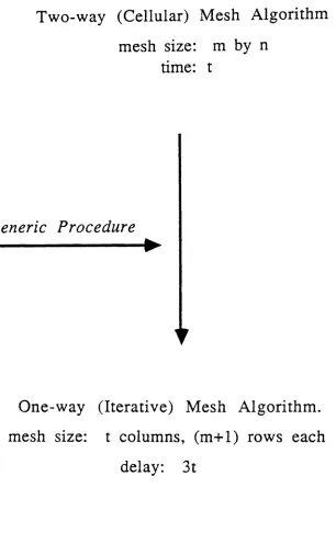
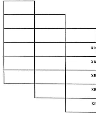
In this paper, we describe a generic procedure to transform any algorithm for a cellular mesh with two-way data flow between adjacent cells into an algo-rithm for an iterative mesh model with only one-way data flow between adja-cent cells [Figure 1]. Precisely, we show how a two-way mXn cellular mesh, computing for t time units, can be simulated by a one-way iterative mesh with

t columns of m +1 rows each: input columns enter the iterative mesh in suc-cessive time units and, after a delay of 3t time units, output columns leave the

mesh in successive time units [Figure 2]. Further, successive problem instances can be pipelined, allowing the possibility of processing a sequence of input arrays (e.g. images) at transmission rates. We discuss the practical implications

of this result for two-dimensional signal processing and the relationship to some

open theoretical questions.

We use the term mesh to refer to a two-dimensional array of processing

elements, each connected to its four nearest neighbors. Operation of the mesh

isdescribed in terms of a cell program which defines the state of a cell at time t

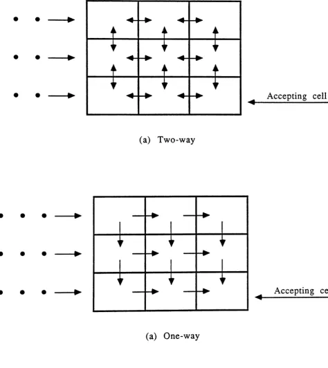
as a function of the states of the cell and its neighbors at the previous time unit [Figure 3]. If the mesh has two - way data flow, the neighbors of a cell are

those cells above, below, left, and right [Figure 3{a)]. In a mesh with

one - way data flow, a cell has only the cells above and to the left as neighbors

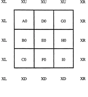
consist of an m Xn array of values. In this paper, we call a computation on an mXn mesh cellular if for 1 < i -s m, 1 < J. < n, cell (i,j) of the array stores input item (i,j) at the beginning of the computation and holds output item (i,j)

at the end of the computation [Figure l{a)]. During the computation, there is

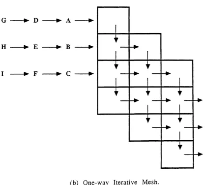
no I/O. We will call a mesh computation iterative if the input enters the mesh, one column per time unit, at the leftmost column of the mesh and the output leaves the mesh one column per time unit, at the rightmost column of the mesh

[Figure l(b)].

In the case of linear arrays, several researchers have made the observation

that a two-way linear cellular array, computing for t time units, can be simu-lated by a one-way linear iterative array with O( n

+

t)

cells [2, 6]. For the case

of the two-dimensional mesh, the only related work of which we are aware is that of [2] which simulates a two-way cellular mesh by a one-way circular

cellu-lar mesh. Simulation by a one-way iterative array uses a different technique and appears to have different applications.

In Section 2, a description is given of the simulation of a two-way cellular

2. The Transformation:

In this section we give an informal description of the simulation of a two-way cellular mesh, P, by a one-way iterative mesh, Q. For convenience in describing the procedure, we assume that P is surrounded by a border of

con-stant values, as shown in Figure 7(a), so that the cell program,

I,

of P is a function of the four neighbors of cell

(i,j)

even when i=l,ffi or j=l,n. (For an

m X n array, P, this will require that each column of Q use m

+

3cells rather than m

+

1 as stated in Figure 2.)

Columns of the initial states of P enter iterative array Q, one column per

time unit. Let P_t(i,;0) denote the state of cell (i,j) of P at time t. In the simu-lation, a cell of Q waits until it has enough information to compute

P,

(i,J

O

) for

some i,

i,

and t. Enough information is saved by the cell so that with its new

input at the next time unit,

P,(i

.i

+

1)can be computed.

Precisely, we can show that all computations performed In array P at

time

t

are performed in column t of Q by cells (t+2, t) ... (t+n+l, t). Further,

column t of Q computes the

ill

column of P at time 3t

+

j. If array P

com-putes for a total of

t*

time units, it follows that the final states of P, Pt., leave

column t- of

Q

in successive time units 3t-

+

1through 3t*

+

n, one column of

P_{t -} per time unit.

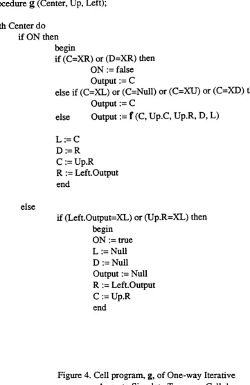
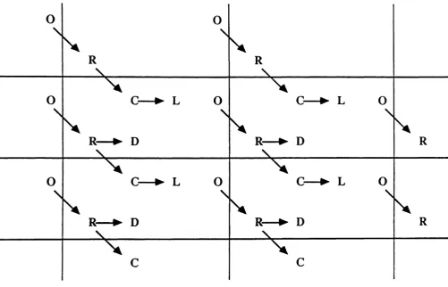
Q holds four values C, L, R, and D, not including the output value it

com-putes. Figure 5 illustrates the flow of data in Q described by the cell program

9 of Figure 4. We omit the details of the formal proof that array Q with cell program g correctly simulates array P with cell program

I

which verifies that all boundary cases do work correctly.

Figure 6 illustrates how and when a neighborhood of cell (i,j) in array P at

time t will show up in array Q. Figure 7 shows the one-way iterative array simulation of a 3

x

3 two-way cellular array, P, computing for 3 time units. In

We begin this section with the disclaimer that the transformation of Section 2 in no sense guarantees optimal one-way solutions on the iterative mesh. With knowledge of the problem at hand, data stored in the simulating array could be substantially pruned. Or, knowing the problem at hand and knowing that a one-way iterative array solution exists,

a designer may start from scratch to devise a clever solution, entirely unrelated to the transformation.

On the other hand, the transformation described in Section 2 proves that any prob-lem whose solution can be described as a cellular mesh computation can be solved on an

iterative mesh with one-way data flow and further that successive problem instances (separated by two columns of "null" values) can be pipelined. This suggests a natural approach to processing sequences of two-dimensional signals at transmission rates.

Image Proeeselngs

Consider the application of processing 512 x 512 images transmitted at video rates:

30 frames per second. A local image operation such as median smoothing might be described by the following cell program for a cellular mesh P: "replace the value of cell

(pixel)

(i,j)

by the median of its current value and those of its nearest neighbors". The

cells of the mesh would execute their program a small number of times k , depending on

the size of the neighborhood over which smoothing is to occur. However, rather than

per-form this computation on a 512

x

512 cellular mesh, the transformation described in

Sec-tion 2 shows that the computaSec-tion can be simulated on an iterative mesh Q of k columns,

3. Applications and Observations:

We begin this section with the disclaimer that the transformation of

Sec-tion 2 in no sense guarantees optimal one-way soluSec-tions on the iterative mesh. With knowledge of the problem at hand, data stored in the simulating array

could be substantially pruned. Or, knowing the problem at hand and knowing

that a one-way iterative array solution exists, a designer may start from scratch to devise a clever solution, entirely unrelated to the transformation.

On the other hand, the transformation described in Section 2 proves that any problem whose solution can be described as a cellular mesh computation

can be solved on an iterative mesh with one-way data flow and further that successive problem instances (separated by two columns of "null" values) can

be pipelined. This suggests a natural approach to processing sequences of two-dimensional signals at transmission rates.

Image Proeeealngs

Consider the application of processing 512 X 512 images transmitted at video rates: 30 frames per second. A local image operation such as

median smoothing might be described by the following cell program for a

cellu-lar mesh P: "replace the value of cell (pixel)

(i,j)

by the median of its current

value and those of its nearest neighbors". The cells of the mesh would execute

their program a small number of times k , depending on the size of the

computation on a 512 X 512 cellular mesh, the transformation described in

Section 2shows that the computation can be simulated on an iterative mesh Q

of k columns, each with 513 cells, which is a more reasonable number of

proces-sors for small k . Successive images can be pipelined through Q and in order to

meet transmission rates, it must be possible to execute the cell program of Q

within 1 sec./(30*512) :::: 70 microseconds, which is very reasonable, especially

ifthe program is implemented in hardware. For global operations, e.g. region

labeling, we retain the advantage that an iterative array can process at

transmission rates, still allowing a generous 70microseconds to execute the cell

program. However, global operations require time at least c*512 on the cellu-lar mesh and therefore the iterative mesh simulating the cellular computation

will require at least e *512 columns.

So, even global operations on images can be performed at transmission

rates on an iterative mesh

If

enough cells are available.

Recirculating Output:

Assume that P is an mX n two-way cellular mesh with cell program

f ·

Let g be the cell program for the one-way iterative mesh simulation of P which

is described in Section 2. Let R be a one-way iterative mesh with cell program

g and with k columns, each with m

+

1 cells. The output of R can be

recircu-lated to follow the input of R and flow through R again for further processing.

input only one time through an iterative array R' which has the same cell pro-gram as R, but which has ck columns of m+1 cells each. This in turn gives

the same result as the array P executing cell program

f

for ck time units. As a

result, then, a computation on a two-way cellular array, P, which requires t*

time units can be simulated by a one-way iterative array R with k

<

t

columns, of m

+

1 cells each, by recirculating the output of R back through R

for

r(t4r

/k)

1-1

times as long as the following condition is met: For all i,j:

i s i < m, 1 -s j < n, P_{t-(i ,j )= Pk}r(t-lk)l(i ,j ). If k divides

t,

this will

cer-tainly be true. Otherwise, the condition says that if P computes for longer

than necessary, it still gets the same result.

Thus, whenever the condition can be satisfied, solving a problem on a one-way iterative array with too few columns can be handled in a natural way

by recirculating output, thereby avoiding the issue of problem decomposition.

Sortingl

It was first established by Thompson & Kung

(14]

that sorting m*n

numbers could be performed by an m X n two-way cellular mesh in time

O( m

+

n) using, for example, the snake ordering on the mesh. Although the

algorithm of

[14)

was described recursively, the recursion can be "unwound" to

uncover a cell program,

f,

which, when executed repeatedly, for O( m

+

n)

steps, will sort the array. Once the function

f

is obtained, the generic

one-way iterative mesh. What we found most intriguing was the idea that

there might be a more natural way to sort on a one-way iterative array (using at most O( m

+

n) columns of m

+

1cells each). This is related to the open ques-tion of whether or not it is possible to sort on an mX n cellular mesh in time o( m

*

n) [i.e., time strictly smaller, asymptotically, than m*n) using only local operations, as we discuss below.

In the past few years several more algorithms have been discovered for

sorting on an mXn cellular mesh in time O(m+n)

[12,9].

With some work, each of these algorithms can be expressed as a cell program,

I,

which, when

executed by each cell in the array for O( m

+

n) steps, will sort the array. How-ever, each of these algorithms uses a global strategy to sort the array. For example to implement a substep such as "sort all rows", the number of times a particular cell compares with its row neighbors depends on the size of the

array. Note that in the cellular array there is no global control: all control is

encapsulated within the cell state and the cell program. Thus, for example, the cell program for the Thompson and Kung sorting algorithm must tell the cell

how to keep track of enough information so that the cell knows when it is to be

shuffling or merging, swapping or comparing. In a local sorting algorithm, the

neighbor or neighbors to which a cell compares and the action taken as a result

of that comparison is independent of the size of the array. Even the shearsori

cri-terion.

In [7] Kosaraju proposed a local sorting scheme which was shown in [8] to

be at least

n(

n

2)

for an nXn mesh. We proposed a local sorting scheme, wavesort, which we conjectured to be linear, but experimental evidence

indi-cates that it is nonlinear, and probably quadratic. No local sorting algorithm

which is faster than quadratic has been found. On the other hand no one has been able to show that local sorting requires more than linear time.

Aside from the theoretical interest, the existence of a linear time local sort would mean that if the entire cell program were hardwired, two mXn meshes

could be combined to sort 2mn values without changing the cell circuitry.

Because of the two-way to one-way transformation of Section 2, the

existence of a linear time local sort on a cellular mesh would imply the existence of a local sort on a one-way iterative mesh with a linear number of

columns. Perhaps more useful is the converse observation that the nonex-istence of a local sort for m *n values on a one-way iterative array with

O(m+n) columns (of m+1cells each) would imply the nonexistence of a linear time local sort on a cellular mesh. Since the one-way iterative array is a more

Arrays of Finite State Machlness

We have not required cells in the mesh to be finite state machines. How-ever, if the cells of the two-way cellular mesh, P, are finite state machines,

then so are the cells of the one-way iterative mesh Q which simulates P, as described in Section 2. Further, meshes P and Q can be interpreted as accep-tors, where a mesh is said to accept its input if and only if the bottommost cell of the rightmost column ever enters an accepting state.

Linear array acceptors can be classified as either cellular (CA) or iterative (IA) according to whether the input is in the initial states of the cells or enters the first cell of the array, one value per time unit (we use the notation of

[5]).

In addition, linear array acceptors may have either two-way data flow (CA, IA)

or one way data flow (OCA, OIA) between adjacent cells [5]. Linear arrays of length n work on input strings of length n and accept a string if and only if the

rightmost cell ever enters an accepting state.

It is straightforward to show that CA's and lA's are both equivalent to

linear space-bounded Turing Machines and thus are equivalent in computing

power. Not so obvious is the equivalence between the OCA and OIA models,

which was recently shown in [5]. The interesting open question is whether the OCA and CA are equivalent. It has been shown that resolving this question in

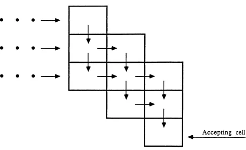
In two dimensions, the cellular and iterative models have been studied

both for two-way data flow (eM) and for one-way data flow (OeM) (3, 4, 10, 11, 15]. It can be shown using techniques from [15] that the two-way mesh

model is strictly more powerful than a one-way mesh using the same number of

cells. (This is in contrast to the result of this paper which allows the number of columns of the one-way mesh to vary with

t.)

In the iterative case, the natural

extension of IA and OIA to 2-dimensions would be the IM and OIM models in Figures Sa and b. In the case of the OIM, it might appear that, for the same number of cells, the iterative mesh model of Figure 9 would be more powerful,

[1]

[2]

[3]

[4]

[5)

[6J

[7]

[8]

[9]

[10]

[11]

[12]

[13]

(14)

References

J.H. Chang, O.H. Ibarra, and A. Vergis, "On the power of one-way communication", Proc, 27th Annual IEEE Symp. on Foundations 01

Computer Science, Toronto, October 1986, 455-464.

K. Culik, and S. Yu, "Translation of systolic algorithms between systems of different topology", Proc. Int. Con]. on Parallel

Process-ing, August 1985, 756-763.

C. Dyer, "One-way bounded cellular automata", Information and Control

44,

1980, 261-281.

F .C. Rennie, Iterative Arrays of Logical Circuits, MIT Press, Cam-bridge, Mass. (1961).

O.H. Ibarra, and T. Jiang, "On one-way cellular arrays", SIAM J.

Computing, Vol. 16, No.6, December 1987, 1135-1154.

A.Z. Kotob, "Transforming computations with hi-directional data flow into ones with uni-directional data flow on linear systolic arrays", Master's thesis, North Carolina State University, 1987. S.R. Kosaraju, "On some open problems in the theory of cellular automata", IEEE Trans. Computers, c-29, 6, June 1974,561-565. R.J. Lipton, R.E. Miller, and L. Snyder, "On an array sorting prob-lem of Kosaraju ", Proe., Conf. on Information Sciences and Sys-tems, The Johns Hopkins University, 1977,99-103.

Y. Ma, S. Sen, and I.D. Scherson, "The distance bound for sorting on mesh connected processor arrays is tight", Proe. 27th Annual IEEE Symp. on Foundations of Computer Science, Toronto, October 1986, 255-263.

A. Rosenfeld, and D.L. Milgram, "Parallel/sequential array

auto-mata", Information Processing Letters 2, 1973, 43-46.

C.D. Savage, "Computing majority on a mesh with one-way dataflow", Information Processing Letters, to appear.

C.P. Schnorr, and A. Shamir, "An optimal sorting algorithm for mesh connected computers", Proe. 8th Annual ACM Symp. on

Theory of Computing, California, May 1986, 255-263.

I.D. Scherson, S. Sen, and A. Shamir, "Shear sort: a true two-dimensional sorting technique for VLSI networks", Proc. Int. Con]. on Parallel Processing, August 1986, 903-908.

Figure 1. Mesh models of computation. (a) Two-way cellular mesh.

(b) One-way iterative mesh Figure 2. Main result.

Figure 3. Cell functions and data flow.

(a) Two-way data flow: cell function computes next state of center

cell as I(C,U,D,L).

(b) One-way data flow: cell function computes next state of center cell as

f (

C, U ,L ).

Figure 4. Cell program, g, ofone-way iterative array to simulate two-way cellular array with cell program

f .

Figure 5. Flow of data in one-way simulation.

Figure 6. Simulation of two-way cellular array, P, by one-way iterative array, Q.

(a)Array P at time

t.

(b) Array Q at time 3(t

+

1)

+

Je - 1.

Figure 7. Simulation of two-way cellular P by one-way iterative Q. (a)Array P at time t=0.

(b) Array

Q

at time

o.

(c)

Array Q at time 1.

(d) Array

Q

at time 2. (e) Array

Q

at time 3.

(f)

Array Q at time 4.

(g)

Array Q at time 5.

(h) Array Q at time 6.

(i)

Array

Q

at time 7.

(j)

Array Q at time 8. (k)Array Q at time 9.

(1)

Array

Q

at time 10. (m) Array Q at time 11.

(n)

Array

Q

at

time 12. (0)Array Q at time 13.

G ~ D

-..

A ~

~,

H ~

E

~ B ~ -...

~, ~,

I ~

F

~

C

~ -...

...

...

~, ~, _~~

...

... ...

.... 'III"""'"

...

~, _~~

... ...

tI"""'"" ...

~,

...

....

(b) One-way Iterative Mesh.

mesh size:

m

by

n

time:

t

Generic Procedure

---~~

One-way (Iterative) Mesh Algorithm.

mesh size:

t

columns, (m+

1)

rows

each

delay:

3t

~,

Left ... Ce n terj.... -... Right

~~

Down

(a) Two-way dataflow: Cell function computes next state of center cell as f(C, U, R, D, L).

Up

~,

Left ... Center....

(b) One-way dataflow: cell function computes next state of center cell as fCC, U, L).

with Centerdo

ifON then begin

if(C=XR) or(D=XR) then ON:= false Output:= C

else

if

(C=XL) or (C=Null) or (C=XU) or (C=XD) then Output:= C

else Output:=

f

(C, Up.C, Up.R, D, L)

L:=C

D:=R C :=Up.R

R

:= Left.Output

end

else

if

(Left.Output=XL) or (Up.R=XL) then begin

ON :=true L:= Null

D :=Null Output:=Null R :=Left.Output C :=Up.R

end

o

o

R

c--.

L

c--.

L

R~D

c

o

o

R

c--.

L

R.-. D

c.-.

L

R~D

c

o

o

R

R

Row i

v

y

u

w

x

(a) Array P at time t

Column

t+l

C L

v

w

u

R D

C L

u

y

Row t+l+i

x

R D

(b) Array Q at time 3(t+ 1)+j-l

Figure 6. Simulation of

Two-way

Cellular Array P

XL

XL

XL

AD

DO

GO

BO

EO

HO

CO

FO

10

XR

XR

XR

XL XD XD XD XR

(a) Array P at time t=O

Figure 7. Simulation of Two-way Cellular

P

XL

_....

...

XL

..

....

XL _...

....

XL _...

....

(b)

Array

Q

at time

0

(c)

Array

Q

at time 1

Figure 7. Simulation of Two-way Cellular P

xu

xu

XU

XR

_....

GO DO XL

...

DO AO Al XR

~ _{00 EO XL}

....

EO 80 Bl XR

...

10 FO XL

...

FO CO Cl XR

~ _{XD XD XL}

...

XD XD XD

XL

(I)

Array

Q

at

time

4

XU XU XU

XR GO XU XL

GO DO Dl _XL

XR 80

At

XL

110 EO EI XL

XR 10 81 XL

10 FO Fl _XL

XR XD Cl XL

XD XD XD XL

XD XL

XL

(g)

Array

Q

at time

5

XR XU XU

XR XU XU

XR GO GI XU XL XL

XR DI Al

XR 00 HI Al XL XL

XR EI 81

XR 10 II 81 XL XL

XR

Fl

CI

XR XD XD Cl XL XL

XD XD

XD XL XL

(h) Array

Q

at time

6

XR

XU XU

XR _XU XU XU

Gl DI XL

XR Dl Al A2

HI El XL

XR El 81 82

II Fl XL

XR FI Cl C2

XD XD XL

XD XD XD

XL

(i) Array Q at time 7

xu

XU XIJ

XR Gl XU XL

Gl Dl D2 XL

XR HI A2 XL

II 1 El E2 XL

XR I 1 82 XL

I 1 Fl F2 XL

XR XD C2 XL

XD XD XD _XL

XD XL

XL

(j)

Array

Q

at

time

8

XR XU XU

XR XU XU

XR Gl G2 XU XL XL

XR D2 A2

XR HI H2 A2 XL XL

XR E2 82

XR 11 12 B2 XL XL

XR F2 C2

XR XD XD _C2 XL XL

XI) _XD

XI) XL XL

(k) Array Q at

time

9

Figure 7. Simulation of Two-way Cellular P

XR

XU

xu

""

XR _XU XU XU

G2 D2

-XR D2 A2 A3

112 E2

XR _E2 82 83

1 2 F2

XR _F2 C2 C3

XD XD

XD XD XD

(I) Array

Q

at

time

10

XU XU

XU XU XU XR G2

G2 D2 D3

XR 82

112 E2 E3

XR 12

1 2 F2 F3

XR XD

XD XD XD

XR

(m)

Array

Q

at

time

11

Figure 7. Simulation of Two-way Cellular P

XR

XR XU XU XR

XR G2 G3

XR

XR 82

_"3

XR

XR I 2 I 3

XR

XR XD XD

XR

(0) Array

Q

at time 12

XR

XR

XR

XR

XR

(0) Array Q at time 13

Figure 7. Simulation of Two-way Cellular P

•

•

•

•

•

•

(a) Two-way

(a) One-way

Figure 8. Iterative Mesh Models

"

•

• •

~ ...

...

~~ ~~

• • •

~ ... ...

-

....

,....

~, ~,

...

...

"

~

Accepting

cell