Computer Simulation Studies of Self-Assembly of Fibril-Forming Peptides with an Intermediate Resolution Protein Model.

ABSTRACT

WAGONER, VICTORIA. Computer Simulation Studies of Self-Assembly of Fibril-forming Peptides with an Intermediate Resolution Protein Model. (Under the direction of Carol K. Hall).

Assembly of normally soluble proteins into ordered aggregates, known as amyloid fibrils, is a cause or associated symptom of numerous human disorders, including Alzheimer's and the prion diseases. Recent experimental studies have offered tantalizing clues regarding the fibril structure, but our understanding of its assembly is still far from complete. The long term goal of our work is to determine the underlying physical forces responsible for the mis-folding and aggregation of proteins. Since the likely toxic species in the various amyloid diseases is believed to occur either on or off the fibrillization pathway, it is of interest to understand the connection between the protein sequence and the structure of the final product, the fibril. The focus here is on short fragments of amyloid proteins; these are believed to be the “Velcro” that holds the fibrillar structures formed by the parent protein together, and can in fact form fibrils themselves.

from the Syrian hamster and mouse prion proteins and variations thereof, and (2) short, truncated amyloid and amyloid-like peptides, some of whose fibril crystal structures have been measured.

We simulate the spontaneous assembly of several short prion and prion-like peptides starting from random initial configurations of random coils. We investigate fibril formation and structure of 48 peptides of palindromic prion sequences, AGAAAAGA (SHaPrP 113-120), VAGAAAAGAV (MoPr 111--120), and related variations, GAAAAAAG, (AG)4, A8, GAAAGAAA, A10, V10, GAVAAAAVAG, and VAVAAAAVAV. We observe that as the chain length and the length of the stretch of hydrophobic residues increase, the ability to form fibrils increases. However as the hydrophobicity of the sequence increases, the ability to form well-ordered structures decreases. Thus, long hydrophobic sequences like VAVAAAAVAV and V10, form slightly disordered aggregates that are partially fibrillar and partially amorphous. Subtle changes in sequence result in slightly different fibril structures.

Computer Simulation Studies of Self-Assembly of Fibril-Forming Peptides with an Intermediate Resolution Protein Model

by

Victoria Allen Wagoner

A dissertation submitted to the Graduate Faculty of North Carolina State University

in partial fulfillment of the requirements for the degree of

Doctor of Philosophy

Chemical Engineering

Raleigh, North Carolina 2010

APPROVED BY:

_____________________________ ______________________________

Carol K. Hall Robert M. Kelly

Committee Chair

_____________________________ ______________________________

ii

DEDICATION

iii BIOGRAPHY

iv

ACKNOWLEDGEMENTS

It is my pleasure to acknowledge all the people who have contributed their wisdom, support and encouragement towards the completion of this thesis.

I would like to thank my advisor and mentor Professor Carol K. Hall for her support, encouragement and wisdom, both professionally and personally. Professor Hall is truly devoted to her students and without her support I would not be defending my PhD today.

I would like to thank Professor Robert M. Kelly and the National Institutes of Health Biotechnology Traineeship for the education and financial support that made part of this research possible. I would also like to thank the U.S. Department of Education Graduate Assistance in Areas of National Need (GAANN) Computational Science Fellowship for providing financial support. Lastly, I would like to thank the National Institutes of Health Research Grant for funding the entire project.

v

who worked with me this last year to take PRIME to the next level and has provided me with gentle guidance and wisdom. I would like to thank Dr. Andrew Schultz and Dr. Steven Smith both of whom developed and improved the discontinuous molecular dynamics simulation method that now allows us to study large macromolecule systems in a reasonable time frame.

I would also like to thank all of my fellow computer system administrators Andrew Schultz, Aysa Akad, Arthi Jayaraman, Alex Marchut, Amit Goyal, Johnny Maury-Evertsz and Ravish Malik, for all of the hard work, time and energy that is required to maintain our computer system of over forty clusters and almost two hundred processors.

I would like to thank Professor Keith Gubbins, Professor Robert Kelly and Professor Clay Clark for serving on my committee and for their advice on my research. I would especially like to thank all of the faculty and staff of NCSU’s Chemical and Biomolecular Engineering Department, and Todd Marcks and Dr. Shaffer of the North Carolina State Graduate School for everything they have done for me while I have been at NC State.

vi

vacations and good times we have shared and for bringing three of the neatest people into this world: my nieces, Kelly and Brittany, and my nephew, Noah. I thank my parents, Sonny and Eva, for allowing me the freedom to reach my goals and for believing that I could do anything. I would also like to thank my in-laws Wayne and Daphna Wagoner who, aside from raising a wonderful son, have embraced me as a daughter and provided me with encouragement to follow my dreams.

vii

TABLE OF CONTENTS

LIST OF TABLES ... xi

LIST OF FIGURES ... xiv

Chapter1. Introduction ...1

1.1 Motivation ...1

1.2 Overview ...4

1.3 References ...8

Chapter 2. Computational Approaches to Fibril Structure and Formation ...11

2.1 Introduction ...11

2.2 Protein Models ...15

2.2.1a All-atom Molecular Dynamics ...16

2.2.1b CHARMM ...17

2.2.1c Simulation Results on Fibril Structure Using All-atom MD ...22

2.2.2a Intermediate-resolution model with Discontinuous Molecular Dynamics ...24

viii

2.2.2c Intermediate Resolution Protein Models – PRIME ...30

2.2.2d Simulation results on fibril formation and structure using DMD ..33

2.3 Conclusions ...39

2.4 References… ...41

2.5 List of Tables ...49

2.6 List of Figures ...50

Chapter 3. Computer Simulation Study of Amyloid Fibril Formation by Palindromic Sequences in Prion Peptides...60

3.1 Introduction ...60

3.2 Methods...67

3.3 Results ...75

3.4 Discussion ...83

3.5 Acknowledgements ...85

3.6 References ...86

3.7 List of Tables ...92

ix

Chapter 4. Understanding the Molecular Assembly of Small Fibril-forming

Peptides: A Computer Simulation Study ...102

4.1 Introduction ...102

4.2 Methods...115

4.3 Results & Discussion ...121

4.4 Conclusions ...132

4.5 Acknowledgements ...133

4.6 References ...134

4.7 List of Tables ...139

4.8 List of Figures ...141

Chapter 5. Future Work ...155

5.1a Improving the representation of protein geometry in PRIME20 ...156

5.1b Refinement of the discontinuous potentials used to describe particularly complex side chains ...157

5.1c Incorporation of solution conditions into PRIME20 by modeling changes in pH ...157

x

xi

LIST OF TABLES

Chapter 1. Introduction ...1

Chapter 2. Computational Approaches to Fibril Structure and Formation ... 11

Table 2.1 DMD Simulation Parameters. ...55

Table 2.2 Auxiliary pair parameters for hydrogen bond potential ...57

Chapter 3. Computer Simulation Study of Amyloid Fibril Formation by Palindromic Sequences in Prion Peptides...60

Table 3.1 PRIME20 Geometric and Energetic Parameters for glycine, alanine, and valine ...94

Table 3.2 Types of structures formed by each sequence at inter-mediate temperatures. The percentages of peptides that are monomers, beta-sheets, amorphous aggregates and fibrils are indicated ...95

Table 3.3 Physical characteristics of fibrils formed by AGAAAAGA, GAAAAAAG, A8, VAGAAAAAGAV, GAVAAAAGAV, and A10 ...96

Chapter 4. Understanding the Molecular Assembly of Small Fibril-forming Peptides: A Computer Simulation Study ...102

xii

Table 4.2 PRIME20 Energetic Parameters for All Twenty Amino Acids ...143 Table 4.3a Percentage of each sequence in monomer, β-sheet, amorphous, and fibril

at low temperatures ...144 Table 4.3b Percentage of each sequence in monomer, β-sheet, amorphous, and fibril

at intermediate temperatures ...144 Table 4.3c Percentage of each sequence in monomer, β-sheet, amorphous, and fibril

at high temperatures ...144 Table 4.4 Molecular arrangement of peptides in β-sheets formed by STVIFE,

STVIIE, VEALYL, MVGGVV, SSTSAA, and SNQNNF at the

temperature corresponding to highest structural order ...150 Table 4.5 Table describing the experimental results of Lopez de la Paz and Serrano

versus PRIME20 simulations at low, intermediate and high T* for each sequence. The * on at high T* for STVIAE indicates that simulations on that sequence at higher temperatures were not complete at the time of printing ...151 Table 4.6a Percentage of each sequence in monomer, β-sheet, amorphous, and fibril

at low temperatures ...152 Table 4.6b Percentage of each sequence in monomer, β-sheet, amorphous, and fibril

at intermediate temperatures ...152 Table 4.6c Percentage of each sequence in monomer, β-sheet, amorphous, and fibril

xiii

xiv

LIST OF FIGURES

Chapter 1. Introduction ...1

Chapter 2. Computational Approaches to Fibril Structure and Formation ...11

Figure 2.1 Summary of the information required by CHARMM at the beginning of a simulation [72] ...51 Figure 2.2 Illustration of the double-layered β-sheet formed by Aβ16-22 and a

snapshot from the CHARMM simulation [40] ...52 Figure 2.3 A) Ribbon diagram depicting the arrangement of the 5 copies of

Aβ(10-40).B) Aβ(10-40) as depicted by CHARMM all-atom

simulations package with residues colored according to type.[42] ...53 Figure 2.4 A general procedure for DMD ...53 Figure 2.5 Flowchart for square-well dynamics. Adapted from Alder and

Wainwright (1959) ...54

Figure 2.6 Geometry of inter-mediate resolution protein model, PRIME, for alanine ...56 Figure 2.7 Backbone hydrogen bonding where the dashed circle represents the

xv

Figure 2.8 Snapshots of 48 peptide system at various reduced times, t*. The simulation proceeds from a random initial configuration at

concentration c=10mM and temperature T*=0.14 until the formation of a protofilament at t*=205.9 [18] ... 57 Figure 2.9 Geometry of intermediate resolution protein model, PRIME, for

glutamine...58 Figure 2.10 Tube formed during simulation of 24 polyglutamine 16mers [73] ... 58 Figure 2.11 Snapshot of a 48-peptide ordered aggregate obtained from the c=1mM

simulation at T*=0.12 (Wagoner and Hall unpublished)... 59

Chapter 3. Computer Simulation Study of Amyloid Fibril Formation by

Palindromic Sequences in Prion Peptides...60

Figure 3.1 Simulation snapshots of GAVAAAAVAG (left) and VAGAAAAGAV (right) at T*=0.17. Snapshots rendered using VMD...97

Figure 3.2 Simulation snapshot of the SHaPrP 113-120 fibril 3.1 and close up of the arrangement of side chains at the interface between the sheets ...98 Figure 3.3 Snapshot of the AGAAAAGA, rotated image of Figure 3.2 ...99 Figure 3.4 Simulation snapshots for SHaPrP 113-120 at T*=0.15, shown at time,

t=10 (very early), t=400, t=1000 and at the end of the simulation, t=1700 ...100

xvi

Figure 3.5 Population graph for the various species (monomers, β-sheets,

amorphous and fibrils for AGAAAAGA at T*=0.15 ...101 Figure 3.6 Population graph for the various species (monomers, β-sheets,

amorphous and fibrils for VAGAAAAGAV at T*=0.17 ...101 Chapter 4. Understanding the Molecular Assembly of Small Fibril-forming

Peptides: A Computer Simulation Study ...102

Figure 4.1a Simulation snapshot of fibril formed by 48 peptides of STVIIE at T*=0.16 and c=10mM ...145 Figure 4.1b Simulation snapshot of fibril formed by 48 peptides of SNNQNF at

T*=0.13 and c=10mM ...145 Figure 4.2 Population of each species: monomer, β-sheet, amorphous, and fibril

for GGVVIA at T*=0.13 ...146 Figure 4.3 Population of each species: monomer, β-sheet, amorphous, and fibril

for MVGGVV at T*=0.15 ...146 Figure 4.4 Simulation snapshots of 48 peptides of GGVVIA at T*=0.13 and

c=10mM ...147 Figure 4.5 Simulation snapshots of 48 peptides of MVGGVV at T*=0.15 and

c=10mM ...148 Figure 4.6 Population of each species: monomer, β-sheet, amorphous, and fibril

xvii

1

CHAPTER 1

Introduction

1.1

Motivation

The hallmark of many neurodegenerative diseases, including Alzheimer’s disease, is the accumulation and deposition of protein plaques in specific tissues within various organs in the body [1]. These plaques are composed of ordered protein aggregates known as amyloid fibrils which form when normally-soluble disease-specific proteins undergo a conformational change that leads to their aberrant assembly. Many of the twenty-four known so-called amyloid diseases are fatal.

In vitro experiments on the many different proteins associated with amyloid diseases, e.g. β-amyloid (Alzheimer’s), prion protein (transmissible spongiform

2

hydrogen bonds to form β-sheets parallel to the fibril axis. Interestingly, proteins other

3

4

This thesis describes research aimed at using computer simulations to develop an understanding of protein aggregation into amyloid fibrils. We have developed a new implicit solvent force field, PRIME20, to describe the geometry and energetics of all twenty amino acids [20]. We use discontinuous molecular dynamics computer simulation to explore the self-assembly and structure of homogeneous systems of known amyloid fibril peptides in an attempt to elucidate the role of peptide sequence and backbone in fibril formation.

1.2

Overview

In this section, we summarize the remaining chapters of this thesis. All chapters contain their own literature review and bibliography.

5

Chapter 3 describes our results for homogeneous systems of truncated aliphatic prion-related sequences. We selected ten different sequences that may or may not form amyloid fibrils to varying degrees based upon the Syrian Hamster prion peptide, SHaPrP 113-120 (AGAAAAGA) and the mouse prion peptide, MoPrP 111-120 (VAGAAAAGAV). The other eight sequences were: GA6G (a longer uninterrupted alanine stretch flanked by glycine), (AG)4 (a complete disruption of the hydrophobic stretch), GAAAGAAA (a mimic of Aβ 28-35), A8, VAVAAAAVAV (a MoPrP with

6

7

Chapters 2, 3 and 4 are adapted from the following publications:

Chapter 2: V.A. Wagoner and C.K. Hall, “Computational approaches to fibril formation and structure”, Methods in Enzymology, 2006. 412: p. 338-365.

Chapter 3: V.A. Wagoner and C.K. Hall, “Computer Simulation of Amyloid Fibril Formation by Palindromic Sequences in Prion Peptides”, in preparation.

8

1.3

References

1. Koo, E.H., P.T. Lansbury, and J.W. Kelly, Amyloid diseases: Abnormal protein aggregation in neurodegeneration. Proc Natl Acad Sci USA, 1999. 96: p. 9989-9990.

2. Blake, C. and L.C. Serpell, Synchotron x-ray studies suggest that the core of transthyretin amyloid fibril is a continuous β-sheet helix. Structure, 1996. 4: p. 989.

3. Sunde, M., et al., Common core structure of amyloid fibrils by synchotron x-ray diffraction. J. Mol. Biol., 1997. 273: p. 729.

4. Chiti, F., et al., Designing conditions for in vitro formation of amyloid protofilaments and fibrils. Proc. Natl. Acad. Sci. USA, 1999. 96: p. 3590.

5. Kelly, J.W., et al., Transthyretin quaternary and tertiary structural changes facilitate misassembly into amyloid. Adv. Protein Chem., 1997. 50: p. 161.

6. Kelly, J.W., Towards an understanding of amyloidogeneisis. Nat. Struct. Biol., 2002. 9: p. 323.

9

8. Monsellier, E. and F. Chiti, Prevention of amyloid-like aggregation as a driving force of protein evolution. European Molecular Biology Organization reports 2007. 8(8): p. 737-742.

9. Fandrich, M. and C.M. Dobson, The behavior of polyamino acids reveals an inverse side chain effect in amyloid structure formation. European Molecular Biology Organizatin, 2002. 21: p. 5682-5690.

10. Nelson, R., et al., Structure of the cross-beta spine of amyloid-like fibrils. Nature, 2005. 435(7043): p. 773-8.

11. Petkova, A.T., W.-M. Yau, and R. Tycko, Experimental constraints on quaternary structure in alzheimer's beta-amyloid fibrils. Biochem, 2006. 45: p. 498-512.

12. Makin, O.S., et al., Molecular basis of amyloid fibril formation and stability. Proc Natl Acad Sci U S A, 2005. 102(2): p. 315-320.

13. Rambaran, R.N. and L.C. Serpell, Amyloid fibrils. Prion, 2008. 2(3): p. 112-117.

14. Tycko, R., Molecular structure of amyloid fibrils: Insights from solid-state nmr. Quarterly Reviews in Biophysics, 2006: p. 1-55.

10

16. Ma, B. and R. Nussinov, Molecular dynamics simulations of alanine rich β-sheet oligomers: Insight into amyloid formation. Prot. Sci., 2002. 11: p. 2335-2350.

17. Nguyen, H.D. and C.K. Hall, Molecular dynamics simulations of spontaneous fibril formation by rando-soil peptides. Proc Natl Acad Sci USA, 2004. 101(46): p. 16180-16185.

18. Hall, C.K., et al., Simulations of protein aggregation: A review, in Misbehaving proteins, R.F. Murphy and A.M. Tsai, Editors. 2006, Springer New York.

19. Hall, C.K. and V.A. Wagoner, Computational approaches to fibril formation and structure. Methods in Enzymology, 2006. 412: p. 338-365.

11

CHAPTER 2

Computational Approaches to Fibril Structure

and Formation

2.1 Introduction

The hallmark of many neurodegenerative diseases, including Alzheimer’s disease, is the accumulation and deposition of protein plaques in specific tissues within various organs in the body [1]. These plaques are composed of ordered protein aggregates known as amyloid fibrils which form when normally-soluble disease-specific proteins undergo a conformational change that leads to their aberrant assembly. Many of the twenty-four known so-called amyloid diseases are fatal. [2-5].

In vitro experiments on the many different proteins associated with amyloid

diseases, e.g. β-amyloid (Alzheimer’s), prion protein (transmissible spongiform

12

itself is a ‘cross-β’ structure with β strands perpendicular to the fibril axis connected by

backbone hydrogen bonds to form β-sheets parallel to the fibril axis. Interestingly,

proteins other than those known to cause one of the amyloid diseases have been found to form fibrils when their protein’s native state is disrupted, such as in the presence of denaturant or under concentrated conditions [11-12]. As a consequence, a number of researchers have begun to think that it is the basic interactions experienced by all proteins e.g., the hydrophobic interactions and hydrogen bonding, rather than the chemistry associated with specific sequences, that drive amyloid formation [3, 11]. This implies that fibril or protofibril [13] formation may be an intrinsic property of many different proteins [4, 14-16] not just those associated with the amyloid diseases.

13

on the complex problem of protein aggregation by studying simple sequences with computer simulations. Important lessons about the essential physical features necessary for the formation and structure of disease-related amyloid fibrils could be learned with the use of computer simulations, provided that the models employed are reasonable representations of the real molecule.

In this paper we focus on the two methods mentioned in the previous paragraph, molecular dynamics simulations based on all-atom protein models and discontinuous molecular dynamics simulation based on intermediate resolution protein models, and their application to protein aggregation. Both methods are rooted in molecular dynamics simulation. In molecular dynamics, the trajectories of studied atoms are computed by solving Newton's equation of motion at regularly spaced time intervals, called time steps. At the beginning of each time step the net force acting on each molecule due to all the other molecules is calculated. Knowledge of this force allows the determination of each molecule's acceleration (F=ma), which in turn allows the prediction of the position and velocity of each molecule at the beginning of the next time step. At each time step, the instantaneous values of thermodynamic properties are computed and recorded. Thermodynamic properties are obtained by averaging the instantaneous properties over time. [19-21]

14

potentials (e.g., hard sphere and square-well potentials). Unlike soft potentials such as the Lennard-Jones potential, discontinuous potentials exert forces only when particles collide, enabling the exact (as opposed to numerical) solution of the collision dynamics. This imparts great speed to the algorithm, allowing sampling of longer time scales and larger systems than traditional molecular dynamics. The particle trajectories are followed by analytically integrating Newton’s equations of motion, locating the time between collisions and then advancing the simulation to the next collision (event) [22-23]. DMD on chain-like molecules is generally implemented using the "bead string" algorithm introduced by Rapaport [24-25] and later modified by Bellemans et al. [26]. Chains of square-well spheres can be accommodated in this algorithm by introducing well-capture, well-bounce, and well-dissociation "collisions" when a sphere enters, attempts to leave, or leaves the square well of another sphere. In canonical ensemble DMD simulations (constant system size, volume and temperature), the temperature is maintained constant by implementing the Andersen thermostat method [27]; all spheres are subjected to random, infrequent collisions with ghost particles whose velocities are chosen randomly from a Maxwell Boltzmann distribution centered at the system temperature.

15

hydrogen bond, the distance between two key amino acids, etc. Structural properties can also be determined such as the radius of gyration which is a measure of the distance of particle i from the center of mass of the entire molecule

Rg* ₌

N z z y y x x

N _iN i c i c i c

2 1

2 2

2 _{( ) ( ) ]}

) [(

/ 1

σ

∑

<

(1)

In addition, knowing the internal energy (E) of the system allows us to calculate many other properties such as the melting temperature, free energy, and the heat capacity

2 * 2 2 * ) ( ] ) ( [ T E E k C C B v v _ε > < − > < = = ₍₂₎

by employing statistical mechanical relationships. These properties can be compared with experimentally-determined properties.

2.2 Protein Models

16

a simulation. The longest all-atom simulation to-date was a 1 μs simulation of the 36

residue villin headpiece starting from an initial configuration with some native state characteristics performed by Duan and Kollman [33]. (In comparison the time scale required for a protein to fold from a random coil is 10 – 100 μs [21].) This simulation took two full months on 256 dedicated parallel supercomputers yet they only achieved partial folding of the protein. Therefore, to simulate the complete folding process from a random coil configuration to the protein’s native (folded) state, simplified representations (models) of proteins must be used. The big question is: How much detail is enough?

2.2.1a All-atom Molecular Dynamics

17

quantum calculations. The energy is then the summation of the intra and intermolecular interactions between all of the molecules. There are many all-atom molecular dynamics computer programs (CHARMM, AMBER, and ECEPP to name a few). The programs differ primarily in terms of the description of the forces acting on each atom (the forcefield). We will focus on the CHARMM energy function for illustrative purposes.

2.2.1b CHARMM

18

information necessary for calculating the energy of the molecule such as the force constants, the equilibrium bond distance, bond angle, and dihedral angles, and the van der Waals radii. The cartesian coordinates of a particular protein can also be generated from x-ray crystallography data or NMR data provided by the protein databank. CHARMM uses periodic boundary conditions in order to limit the number of particles necessary to model the protein in solution. A summary of the files and information required in CHARMM to calculate the energy of a molecule in a particular conformation is shown in Figure 2.1 [28, 35]. These features are common to all CHARMM codes regardless of the type of simulation being performed.

The next component of CHARMM is the empirical energy function. There are many different forms for the empirical energy function but all can be expressed as a sum of the following types of terms

E = Eb + Eθ + Eφ + Eω + EvdW + Eel + Ehb + Ecr + Ecφ . (3)

The terms in the energy function include potential energies for the bond length, Eb, bond angle, Eθ, dihedral angle, Eφ, improper torsions, Eω, electrostatic interactions, Eel,

hydrogen bonding interactions, Ehb, and structural constraints, Ecr and Ecφ. Each term in

19

(Coulomb’s Law), a distance-dependent dielectric, a shifted dielectric, a dielectric that depends on the distance between the center of geometry of the two groups containing electrostatic atoms i and j, or an extended dielectric that is the sum of a constant dielectric term and a second term that accounts for the approximate potential and field at atom i due to all other atoms not connected to atom i by angles and bonds outside a predetermined cutoff radius. [28]

An important consideration in computer simulations of protein folding and aggregation is the treatment of the solvent. There are many different options for representing solvent and/or its impact (e.g., the hydrophobic effect) in CHARMM. One of the most common potentials used in CHARMM to describe water-water interaction is the ST2 potential [28] but other models have been used successfully. The detailed description of water-water interactions that characterizes explicit-solvent all-atom molecular dynamics simulations severely limits the time scale that can be accessed. For example, in simulating a single protein molecule solvated with 3000 water molecules most of the computational time is dedicated to keeping track of the water-water interactions. The point is that all-atom explicit-solvent calculations are very expensive computationally and significantly reduce the accessible time scales even for a single protein.

20

effect and electrostatic screening effects. One popular implicit-solvent model is the CHARMM PARAM19 model [36-37]. In the CHARMM PARAM19 model the potential of mean force is described as the sum of both the intra-solute interactions and a mean solvation term. The solvation term is the sum over all the atoms of the product of an atomic solvation parameter and the solvent-accessible surface area [37]. This model assumes that the major contributor to the solvation energy is the interaction between the protein and its first shell of solvent molecules [38]. In an effort to increase computational speed, Ferrara et al. used an approximate method developed by Hasel and coworkers [39] to obtain an analytical expression for the solvent accessible surface area. Additionally, this model enforces a free energy penalty when a charged residue is buried in the protein interior and accounts for electrostatic screening effects with a distance-dependent dielectric. The CHARMM PARAM19 implicit-solvent model is much faster computationally than the explicit-solvent models and requires a mere 50% increase in computational time as compared to in vacuo simulations [37]. However, even with the use of an implicit-solvent model, the timescales accessible in all-atom protein simulations are limited because of the molecular detail of the model.

21

has five different energy minimization techniques: steepest descent (SD), conjugated gradient (CONJ), Powell (POWE), Newton-Raphson (NRAP), and truncated-Newton minimization package (TNPACK). These methods have the common goal of finding a set of coordinates which corresponds to a molecular conformation whose potential energy is at a minimum. [35] Energy minimization can also be used to eliminate structural defects caused by overlapping atoms and distorted bond and torsional angles. Energy minimization is performed not only in the case of a single molecule, but also in the case where the initial configuration is a pre-formed fibril or aggregate structure.

22

reach some biologically relevant time scales, like β-sheet formation, on a system of

parallel supercomputers [33].

2.2.1c Simulation Results on Fibril Structure Using All-atom MD

Nussinov and coworkers have used the CHARMM polar hydrogen force field package in the presence of solvent to monitor the motions of 24 chains of Aβ(16-22), KLVFFAE, initially arranged in a double-layered antiparallel β-sheet configuration[40]. At the end of a 2.5 ns simulation these short highly hydrophobic sequences formed a double-layered β-sheet conformation. The strands within each β-sheet were antiparallel to each other with a 15° twist as shown in Figure 2.2. A more recent study by Haspel and coworkers on systems containing six or nine copies of a short sequence of the amyloidogenic human calcitonin hormone peptide (15-19) [41], DFNKF, led to the observation of a stable parallel β-sheet conformation in a single sheet layer.

23

were chosen to allow for intermolecular backbone hydrogen bonding. The CHARMm forcefield was used to model 5 copies of Aβ1-40 starting from the in-register parallel

(within each β-sheet) cross-β arrangement obtained from the NMR data as described

above and shown in Figure 2.3A. After energy minimization, they observed a fibril structure with the following characteristics: a salt bridge between residues K28 and D23, an offset horseshoe structure for each strand which was held together by intra-chain association of hydrophobic side chains, and inter-chain backbone hydrogen bonding along the fibril axis as shown in Figure 2.3B.

24 antiparallel arrangements.

Atomic resolution simulations have also been used to study destabilizing events that are believed to happen early on during the fibrillization process, such as the α-helix

to β-strand conversion or the partial unfolding of the native state into a conformation

likely to aggregate into ordered structures. Recently, Tarus, Straub and Thirumalai[44] explored the initial stage of aggregation of Aβ10-35, which is thought to be a dimerization based on experimental observations. They used the GRAMM energy minimization program to form two types of dimers, the φ-dimer which is stabilized by hydrophobic

contacts, and the ε-dimer which is stabilized by electrostatic interactions. Each of the

two dimers was then simulated for 10 ns using CHARMM PARAM22 with explicit solvent to determine its structural stability. The φ-dimer did not dissociate while the ε -dimer did, indicating that the expulsion of water molecules due to the interaction between hydrophobic residues on the φ-dimer may play a significant role in its structural stability.

2.2.2a Intermediate-resolution protein model with discontinuous molecular

dynamics

25

aggregation (for example the cross-β structure in protofilaments) seem to be less dependent on the protein sequence than protein folding [11-12]. In fact, Wetzel and coworkers have shown experimentally that mutations in the hydrophobic core of Aβ1-40, residues 17-20, destabilizes the fibril structure but this effect is often counterbalanced by the formation of additional hydrogen bonds [47-48]. These observations suggest that protein aggregation may be less sensitive to the details of the intra-and inter-molecular interactions than protein folding. Therefore, simplified approaches have gained in popularity for studies of aggregation in multi-peptide systems.

There are two avenues by which all-atom molecular dynamics can be simplified. One approach is to change the manner in which the dynamics is calculated, and the secondapproach is to reduce the detail involved in the description of the molecule. These two simplifications can either be used together or separately. In our group’s work we do both. We simplify the dynamics calculation by using discontinuous molecular dynamics and we reduce the detail in the protein’s representation by using an intermediate resolution protein model.

2.2.2b Discontinuous Molecular Dynamics

26

number of molecules in the box, σ is the particle diameter, and V is the volume of the

simulation box. In protein simulations one more commonly refers to the concentration of the system which is given by c = N/L3 where L is the simulation box length. The temperature is set according to the equipartition theorem which relates the system kinetic energy to the temperature

(

)

1 2 _{= (4)}

where m is the particle mass, v is the particle velocity, and kB is the Boltzmann constant.

As mentioned previously, the velocities are assigned randomly from a Maxwell-Boltzmann distribution about the system temperature. Protein aggregation simulations are often performed in the canonical ensemble, which means that the number of particles, volume, and temperature are held constant. Constant temperature is maintained by implementing the Anderson thermostat method [27].

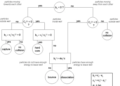
The key steps in a DMD simulation are the calculation of collision times, tij, between particles i and j, and the calculation of the post-collision velocities for the colliding pair. DMD proceeds by calculating the collision times for all possible pairs of particles, determining which collision pair, i and j, has the smallest collision time, advancing the system to that event, and computing the system dynamics. A simple procedure for DMD is shown in Figure 2.4. For two particles, i and j, with diameter σ

27

| rij(t+tij) | = | rij + vijtij | = σ (5)

where rij = ri - rj and vij = vi – vj. The collision time tij is obtained by squaring equation (5) and solving the resulting quadratic equation

2

2 2 2

2 _{( )}

ij ij ij ij ij ij v r v b b

t = − ± − −σ (6)

where bij is defined as bij = rij·vij. This equation must meet certain criteria for the calculated tij to be correct. If bij is greater than 0 then the spheres are moving away from each other and no collision will occur. If bij is less than 0 and the square-root discriminant is positive (to give a real solution) the spheres will collide [22-23, 49]. Equation 6 can be used to generate a list of all collision times for all possible colliding pairs, i and j. The next collision time tc is the minimum collision time in this list. The system is advanced by tc to the new position ri(t+tc), at which a single pair of particles is in contact preparing to undergo a collision

ri(t + tc) = ri(t) + vitc . (7)

After the collision occurs, the post-collision velocities are calculated. The new velocities for interacting particles i and j are determined by imposing conservation of kinetic energy and conservation of linear momentum. The new velocities are given by

vi(after)=vi(before)+∆vi (8)

vj(after)=vj(before)−∆vi (9)

where vi represents each component of the velocity vector and the velocity change, Δvi,

28

vi vj 2rij      − = ∆ − = ∆ σ ij b

. (10)

After each event between partners i and j, the collision time list is updated for particles i and j and any other particles that would have interacted with either i or j. [22, 50]

The equations described thus far are applicable to hard sphere particles undergoing a core collision. Real intermolecular potentials, however, include not just repulsive interactions (like the hard sphere case) but also attractive interactions. The square-well potential is one such potential that has a repulsive interaction at short distances and an attractive interaction at intermediate distances. The square-well potential is mathematically described as,

     > ≤ ≤ − < ∞ = ) σ r ( 0 ) σ r σ ( ) σ r ( ) ( 2 2 1 1 ε ij

U r . (11)

The equations described above for hard sphere particles can easily be extended to the case of the square-well potential [22].

29

that shown in Figure 2.4. The collision times are functions of the separation σ1 or σ2, resulting in slightly different formulas for calculating the collision times and the velocity changes. Alder and Wainwright provide a detailed flow-chart that can be used to determine which type of collision (event) will take place between two interacting particles, i and j. This is reproduced in Figure 2.5 [22]. Additionally, in DMD we have pseudo-events for bookkeeping purposes. These pseudo-events include implementing the thermostat, implementing efficiency techniques, and data collection.

30 2 2 2 2 2

2 _{( (1 ) )}

ij ij ij ij ij Bond ij _v l r v b b

t = − + − − +δ (12)

where (1+δ)l represents the maximum bond length.

The execution speed of DMD is proportional to N2 _{but there are several efficiency} techniques developed by Smith et al. that can be utilized to reduce the execution speed to be proportional to N. See Smith et al. (1997) for a more detailed discussion.

2.2.2c Intermediate Resolution Protein Models – PRIME

Inspired by the early reduced representation model of Takada [51], our group developed an intermediate-resolution protein model for simulations of protein folding and aggregation [52-54]. In this model, which we now call PRIME (for Pr

Resolution Model) the protein backbone is represented by three united atom spheres, one for the amide group (NH), one for the carbonyl group (CO) and one for the alpha-carbon and its hydrogen (CαH). The side chains are modeled with a single sphere of variable

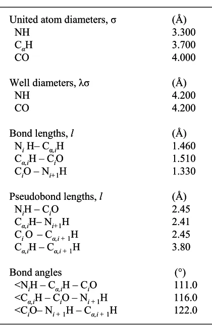
size. All backbone bond lengths and angles are set to their ideal values. As mentioned earlier for DMD on chain-like molecules, the covalent bonds are maintained with a hard sphere interaction occurring when the bond lengths move outside of the range (1+δ) l to (1-δ) l, where l is the ideal bond length and δ is the tolerance for acceptable fluctuation in bond lengths which is set at 2.375% [26]. The covalent bond lengths in this model are given in Table 2.1. Ideal backbone bond angles, Cα-Cα distances and residue

L-isomerization are fixed through a series of pseudobonds which are also allowed to

31

fluctuate within 2.375% of their given length. A depiction of the protein model for alanine showing the backbone united atoms, NH, CαH, and C=O, and side chain united

atom, CH3, along with the covalent bonds and pseudobonds is given in Figure 2.6. The values of bond angles and pseudobond lengths are also given in Table 2.1. Local interactions between united atoms separated along the protein backbone by three or fewer onds are modeled in a similar manner to nonlocal interactions but with different bead diameters. Takada et al. found that it was more appropriate to describe the local interactions with the real atomic diameters (N, Cα, C) rather than the united atom

diameters given in Table 2.1. In order to account for the interactions between atoms connected by three or fewer bonds, we allow 25% overlap of their united atom bead diameters. This treatment of local interactions successfully limits the motion of the phi and psi dihedral angles, yielding reasonable Ramachandran plots [51, 53]. Additionally in PRIME, the side chain can either be represented with a single sphere, as in the case of alanine, or by several spheres, as in the case of glutamine; glycine is incorporated into the alpha carbon united atom and therefore not represented as a sphere.

32

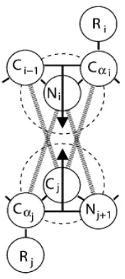
and (3) neither the NH nor the C=O are already involved in a hydrogen bond with a different partner. In order to ensure that criteria 1 and 2 are satisfied we require that the four atom pairs Ni – Cαj, Ni – Nj+1, Cj – Cαi, Cj – Ci-1 shown connected by thick dashed

lines in Figure 2.7 (hereafter referred to as auxiliary pairs), be separated by a distance greater than dij which is chosen to maintain the hydrogen bond angle constraints [55-56]; their values are given in Table 2.2. Upon the formation of a bond between Ni and Cj, these auxiliary pairs temporarily interact via a square-shoulder potential:

     > ≤ ≤ < ∞ = ) r ( 0 ) d r σ ( ) σ r ( ) ( ₁ d

U rij εHB (13)

where r is the distance between spheres i and j; σ is the sphere diameter; εHB is the

shoulder height (equal to the well depth of the hydrogen bond between Ni and Cj) and dis the square-shoulder width. These auxiliary pairs return to their original interactions when the hydrogen bond is broken.

The solvent molecules are modeled implicitly via a square well attraction (potential of mean force) between two hydrophobic residues, and a hard sphere repulsion between two polar residues or between a polar and a hydrophobic residue. The depth of

the square well attraction, εHP, between two hydrophobic residues is scaled relative to εHB

by a factor R, which describes the solvent characteristics of the system [55]; R is defined

as εHP/ εHB. All system parameters are scaled by εHB, so that the system reduced

33

2.2.2d Simulation results on fibril formation and structure using DMD

We performed simulations on a single model polyalanine sequence, Ac-KA14K-NH2 [55]. Polyalanine was chosen for study because Ac-KA14K-Ac-KA14K-NH2 forms fibrils in vitro as shown by Blondelle and coworkers [45]. We began by exploring how the temperature and hydrophobic interaction strength, as modeled through the parameter R, affected the conformational conversion of the isolated chain. At low temperatures and low hydrophobicity (0 < R < 1/10) we observed a transition from an α-helix to random coils. However, as the hydrophobic interaction strength was increased (1/4 < R < 1/2), a third conformational transition from an α-helix to a β-sheet structure was observed. In that case as the temperature increased, the isolated peptide adopted an α-helix, then a β -hairpin or β-sheet and finally a random coil configuration. Finally, at high hydrophobic interaction strength (R > 1/2), the model polyalanine formed only random coils. Since

there is little evidence to support a three state transition (α-helix β-hairpin  random

coils), a value of R was chosen low enough to avoid the three state transition but yet high

enough so that the most stable state at a low temperature is an α-helix.

34

concentrations, and solvent strengths, we determined that as temperature and concentration were increased the number of α-helices decreased and the number of extended ordered structures increased. The protofilament or fibril was found to be stable at temperatures higher than the folding temperature.

We went on to describe the dependence of peptide aggregation on peptide

concentration and temperature by conducting equilibrium simulations using the replica-exchange technique [57] on a system containing 96 16-mers of Ac-KA14K-NH2. A phase diagram in the temperature--concentration space was mapped out, illustrating which structures were stable at each condition [58]. The α-helical region was stable at low temperatures and low concentration. The non-fibrillar β-sheet region was stable at intermediate temperatures and relatively low concentrations and expanded to higher temperatures as concentration was increased. The fibril region was primarily stable at intermediate temperatures and intermediate concentrations and expanded to lower temperatures as the peptide concentration was increased. Finally, the random coil region was stable at high temperatures at all concentrations. Interestingly, we were able to observe the formation of small fibrils (protofilaments) for systems containing 96 peptides within 160 h on an AMD Athlon MP2200+ workstation.

35

formation was a nucleation dependent event. In the presence of a seed (a preformed aggregate) the lag time, which is the time to form a fibril or fibril component, disappeared. The lag time decreased with increasing temperature and concentration. Fibril formation proceeded in the following way: small amorphous aggregates associated, rearranged into ordered β-sheet structures and ultimately formed a “nucleus”, which rapidly grew into a small fibril or protofilament. We observed two growth mechanisms: lateral addition in which a β-sheet was added to the side of the fibril, and end-to-end growth in which individual peptides were attached to the end of each β-sheet (this mechanism accounts for the indeterminate length of the fibril). Once the fibrillar structure reached a critical number of β-sheets, the monomeric peptides tended to attach

to an already formed β-sheet rather than to form a new isolated β-sheet. The number of

critical β-sheets was a function of system size. A 12 peptide system formed a fibril with

2-3 β-sheets, a 24 peptide system formed a fibril with 3-4 β-sheets, a 48 peptide system formed a fibril with 3-6 β-sheets and a 96 peptide system formed a fibril with 4-6 β -sheets.

We have extended the PRIME model to polyglutamine to study the aggregation of polyglutamine-containing proteins [60]. The backbone of a polyglutamine residue is modeled with the same level of detail as a polyalanine residue (a single sphere for the carbonyl group, amide group, and alpha-carbon group). The difference between the polyglutamine and polyalanine models is in the description of the side chain. The

36

hydrophobic methyl groups (CH2, in blue), one for the carbonyl group (CO, in red) and one for the amine group (NH, in green) as shown in Figure 2.9. The carbonyl and amine groups along the side chain allow the side chain to participate in hydrogen bonding either with the backbone amide or carbonyl groups or with other side chains. Simulations were conducted on a system of 24-16 mers (Q16) at a concentration of 5 mM over a range of temperatures starting from a random initial configuration. Amorphous aggregates were formed at low temperatures, annular structures composed of β-sheets were formed at intermediate temperatures, and random coil configurations were found at high temperatures. Figure 2.10 shows a snapshot of one of the annular structures. Similar annular structures were observed by Wacker and coworkers on two cleavage products of the huntingtin protein with 20 and 53 polyglutamine repeats, respectively [61] using atomic force microscopy and were also predicted by Perutz from x-ray scattering data on D2Q15K2 [62].

37

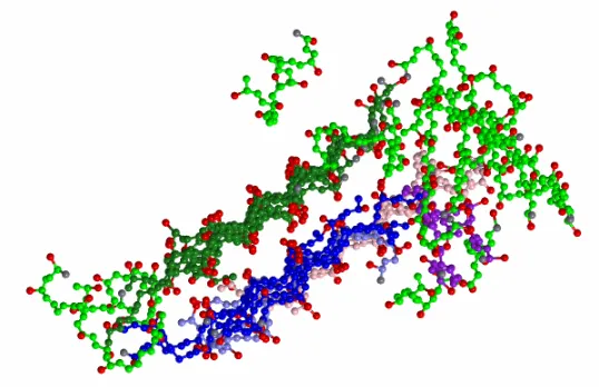
T*=0.07 -- 0.14, and a hydrophobic interaction strength, R=1/10, starting from a configuration of random coils. Amorphous aggregation is observed at or below T*=0.11. Ordered aggregates are formed at temperatures greater than T*=0.11 but less than T*=0.13. The ordered aggregates are composed of stacks of four to six β-sheets. The peptides remain in random coil configurations at temperatures greater than or equal to T*= 0.13. We have also conducted simulations at concentrations, c = 1 mM, 2.5 mM and 10 mM at reduced temperature, T* = 0.12. The peptides formed β-sheets at concentrations greater than c = 1 mM but less than c = 5 mM, and formed ordered aggregates (a protofilament) at concentration, c = 10 mM. Figure 11 is a snapshot of an ordered aggregate formed by a 48 peptide system of VAGAAAAGAV at concentration, c = 1 mM and reduced temperature, T* = 0.12 where peptides which form a β-sheet are colored the same. For example, in Figure 2.11 there are two β-sheets formed, green and blue, respectively, which then associate to form an ordered aggregate.

The great speed of DMD simulations with reduced representation protein models has inspired other groups to develop protein models based upon hard sphere and square well interactions. Dokholyan and coworkers have applied DMD to the study of a two-sphere per residue coarse-grained protein model [63-64] with a Go-type potential used to describe the intermolecular interactions between the side chains. Ding et al. [64] used this two-sphere model to study the aggregation of a system containing eight copies of the Src SH3 protein. Starting from a system of random coils, they observed a possible

38

of four proteins  one aggregate. Peng et al. [65] applied the two-sphere model to study

a large system of β-amyloid proteins, Aβ1-40. They started with 28 copies of the peptide

arranged randomly, with each peptide in a α-helical conformation as determined by the

NMR measurements of Coles et al. [66], at concentration c = 6 mM. They observed the formation of amorphous aggregates at temperatures below the melting temperature of a single peptide, T*=0.4 and dissociation of all structures at temperatures greater than T* =

1.10. Multilayer β-sheet structures formed over a range of simulation temperatures

between T* = 0.55 and T* = 1.10.

Recently, Urbanc et al. [67-68] used a model similar to the four-sphere intermediate resolution model introduced by Smith and Hall [53-54] along with DMD to study the oligomerization of amyloid β-protein, Aβ1-40 and Aβ1-42. They observed an α

-helix to β-strand structural transition at intermediate simulation temperatures followed by

another transition from β-strand to random coil at relatively high simulation temperatures.

They also observed a β-turn between residues D23 and K28. Although a turn is observed

experimentally between residues D23 and K28, it is not a true β-turn (which would

involve hydrogen bonding between residues D23 and K28) but rather an electrostatically driven salt-bridge which leaves the backbone amide and carbonyl groups free to

hydrogen bond with another Aβ1-42 peptide [42]. Urbanc et al. [67] went on to study the

aggregation of 32 copies of Aβ1-40 and Aβ1-42 starting from a mostly α-helical

39

pentamer. The cores of both oligomers were comprised primarily of hydrophobic residues. The observation of the pentamer is interesting because experiments suggest that the composition of protofibrils or paranuclei is predominantly pentameric and hexameric [69-70]. While they were able to see the formation of oligomers, their simulation time was too short to observe the formation of the fibril structure reported by Petkova et al. [71].

2.3 Conclusion

40

experimental tools) that we use afford us views of different aspects of fibril formation. It is only by sharing this information and piecing together our various observations that we will be able to assemble a good comprehensive picture of the nature of fibril formation and structure.

41

2.4 References

1. Koo, E.H., The β-amyloid precursor protein (app) and alzheimer's disease: Does the tail wag the dog? Traffic, 2002. 3: p. 763-770.

2. Bucciantini, M., et al., Inherent toxicity of aggregates implies a common mechanism for protein misfolding diseases. Nature, 2002. 416: p. 507.

3. Dobson, C.M., The structural basis of protein folding and its links with human disease. Phil. Trans. R. Soc. Lond. B., 2001. 356: p. 133.

4. Kelly, J.W., The alternative conformations of amyloidogenic proteins and their multi-step assembly pathways. Curr. Opin. Struct. Biol, 1998. 8: p. 101.

5. Prusiner, S.B., Prion diseases and the bse crisis. Science, 1997. 278: p. 245-251.

6. Sunde, M. and C.C.F. Blake, The structure of amyloid fibrils by electron microscopy and x-ray diffraction. Adv. Protein Chem., 1997. 50: p. 123.

7. Sunde, M., et al., Common core structure of amyloid fibrils by synchotron x-ray diffraction. J. Mol. Biol., 1997. 273: p. 729.

8. Blake, C. and L.C. Serpell, Synchotron x-ray studies suggest that the core of transthyretin amyloid fibril is a continuous β-sheet helix. Structure, 1996. 4: p. 989.

9. Serpell, L., et al., The protofilament substructure of amyloid fibrils. J. Mol. Bio., 2000. 300: p. 1033-1039.

42

11. Chiti, F., et al., Designing conditions for in vitro formation of amyloid protofilaments and fibrils. Proc. Natl. Acad. Sci. USA, 1999. 96: p. 3590.

12. Chiti, F., et al., Solution conditions can promote formation of either amyloid protofilaments or native fibrils from the hypf n-terminal domain. Prot.Sci., 2001. 10: p. 2542.

13. Caughey, B. and P.T. Lansbury, Protofibrils, pores, fibrils, and neurodegeneration: Separating the responsible protein aggregates from the innocent bystanders. Annu. Rev. Neurosci., 2003. 26: p. 267-298.

14. Kelly, J., Amyloid fibril formation and protein misassembly: A structural quest for insights into amyloid and prion diseases. Structure, 1997. 5: p. 595-600.

15. Rochet, J.C. and P.T. Lansbury, Amyloid fibrilogenesis: Themes and variations. Curr. Opin. Struct. Biol., 2000. 10: p. 60.

16. Hou, L. and M.G. Zagorski, Sorting out the driving forces for parallel and antiparallel alignment in the aβ peptide fibril structure. Biophys J, 2004. 86: p. 1-2.

17. Ma, B. and R. Nussinov, Molecular dynamics simulations of alanine rich β-sheet oligomers: Insight into amyloid formation. Prot. Sci., 2002. 11: p. 2335-2350.

18. Nguyen, H.D. and C.K. Hall, Molecular dynamics simulations of spontaneous fibril formation by rando-soil peptides. Proc Natl Acad Sci USA, 2004. 101(46): p. 16180-16185.

19. Frenkel, D. and B. Smit, Understanding molecular simulation: From algorithms to applications. 2nd ed. 1996, Chestnut Hill, MA: Academic Press.

43

21. Leach, A.R., Molecular modelling: Principles and applications. 2nd ed. 2001: Pearson Education Limited.

22. Alder, B.J. and T.E. Wainwright, Studies in molecular dynamics, i: General method. J Chem Phys, 1959. 31: p. 459-466.

23. Smith, S.W., C.K. Hall, and B.D. Freeman, Molecular dynamics for polymeric fluids using discontinuous potentials. Journal of Computational Physics, 1997. 134: p. 16.

24. Rapaport, D.C., Molecular dynamics study of polymer chains. J. Chem. Phys., 1979. 71: p. 3299.

25. Rapaport, D.C., Molecular dynamics simulation of polymer chains with excluded volume. J. Phys. A, 1978. 11: p. L213.

26. Bellemans, A., J. Orbans, and D.V. Belle, Molecular dynamics of rigid and non-rigid necklaces of hard disks. Mol. Phys., 1980. 39: p. 781-782.

27. Andersen, H.C., Molecular dynamics simulation at constant temperature and / or pressure. J. Chem. Phys., 1980. 72: p. 2384.

28. Brooks, B.R., et al., Charmm: A program for macromolecular energy minimization and dynamics calculation. J. Comp. Chem., 1983. 4: p. 187.

29. Weiner, S.J., et al., An all atom force field for simulations of proteins and nucleic acids. J. Comp. Chem., 1986. 7: p. 230.

30. Dauber-Osguthorpe, P., et al., Structure and energetics of ligand binding to proteins: Esherichia coli dihydrofolate reductase trimethoprim, a drug receptor system. Proteins: Struct. Funct. and Genet., 1988. 4: p. 31.

44

32. Zimmerman, S., et al., Conformational analysis of the 20 naturally occurring amino acid residues using ecepp. Macromolecules, 1977. 10(1): p. 1-9.

33. Duan, Y. and P.A. Kollman, Pathways to a protein folding intermediate observed in a 1-microsecond simulation in aqueous solution. Science, 1998. 282: p. 740.

34. Khurana, R., et al., Partially-folded intermediates as critical precursors of light chain amyloid fibrils and amorphous aggregates. Biochemistry, 2001. 40: p. 3525.

35. Molecular Simulations, I., Charmm principles. 1999, San Diego: Inc., Molecular Simulations.

36. Gsponer, J., U. Haberthur, and A. Caflisch, The role of side-chain interactions in the early steps of aggregation: Molecular dynamics simulations of an amyloid-forming peptide from the yeast prion sup35. Proc Natl Acad Sci USA, 2003. 100(9): p. 5154-5159.

37. Ferrara, P., J. Apostolakis, and A. Caflisch, Evaluations of a fast implicit solvent model for molecular dynamics simulations. Proteins: Struct. Funct. and Genet., 2002. 46: p. 24-33.

38. Roux, B. and T. Simonson, Implicit solvent models. Biophysical Chemistry, 1999. 78: p. 1-20.

39. Hasel, W., T. Hendrickson, and W. Still, A rapid approximation to the solvent accessible surface areas of atoms. Tetrahedron Computational Methodology, 1988. 1: p. 103-116.

40. Ma, B. and R. Nussinov, Stabilities and conformations of alzhemier's β-amyloid peptide oligomers (aβ16-22, aβ16-35, and aβ10-35):Sequence effects. Proc Natl Acad Sci USA, 2002. 99: p. 14126.

45

42. Petkova, A.T., et al., A structural model for alzheimer's β-amyloid fibrils based on experimental constraints from solid state nmr. Proc Natl Acad Sci USA, 2002. 99: p. 16742.

43. Santini, S., N. Mousseau, and P. Derreumaux, In silico assembly of alzheimer's aβ16-22 peptide into β-sheets. J Am Chem Soc, 2004. 126: p. 11509-11516.

44. Tarus, B., J.E. Straub, and D. Thirumalai, Probing the initial stage of aggregation of the aβ10-35-protein: Assessing the propensity for peptide dimerization. J Mol Biol, 2005. 345: p. 1141-1156.

45. Blondelle, S.E., et al., Polyalanine-based peptides as models for self-associated β-pleated-sheet complexes. Biochemistry, 1997. 36: p. 8393.

46. Forood, B., et al., Structural characterization and 5'-mononucleotide binding of polyalanine β-sheet complexes. J. Mol. Recognit., 1996. 9: p. 488.

47. Williams, A.D., et al., Mapping abeta amyloid fibril secondary structure using scanning proline mutagenesis. J Mol Biol, 2004. 335(3): p. 833-842.

48. Williams, A.D., S. Shivaprasad, and R. Wetzel, Alanine scanning mutagenesis of abeta(1-40) amyloid fibril stability. J Mol Biol, 2006. 357(4): p. 1283-1294.

49. Smith, S.W., C.K. Hall, and B.D. Freeman, Large scale molecular dynamics study of entangled hard-chain fluids. Phys. Rev. Lett., 1995. 75: p. 1316.

50. Smith, S.W., C.K. Hall, and B.D. Freeman, Molecular dynamics study of transport coefficients for hard-chain fluids. J Chem Phys, 1995. 102: p. 1057-1073.

46

52. Smith, A.V. and C.K. Hall, Protein refolding versus aggregation: Computer simulations on an intermediate resolution model. J. Mol. Biol., 2001. 312: p. 187.

53. Smith, A.V. and C.K. Hall, Α-helix formation: Discontinuous molecular dynamics on an intermediate resolution model. Protein: Structure, Function and Genetic, 2001. 44: p. 344.

54. Smith, A.V. and C.K. Hall, Assembly of a tetrameric α-helical bundle: Computer simulations on an intermediate-resolution protein model. Proteins: Structure, Function and Genetics, 2001. 44: p. 376.

55. Nguyen, H.D., A.J. Marchut, and C.K. Hall, Solvent effects on the conformational transition of a model polyalanine peptide. Prot. Sci., 2004. 13(11): p. 2909-2924.

56. Ding, F., et al., Mechanism for the alpha-helix to beta-hairpin transition. Proteins: Struct. Funct. and Genet., 2003. 53: p. 220-8.

57. Sugita, Y. and Y. Okamota, Replica exchange molecular dynamics method for protein folding. Chem. Phys. Letts., 1999. 314: p. 141.

58. Nguyen, H.D. and C.K. Hall, Phase diagrams describing fibrillization by polyalanine peptides. Biophys J, 2004. 87(6): p. 4122-4134.

59. Nguyen, H.D. and C.K. Hall, Kinetics of fibril formation by polyalanine peptides. J Biol Chem, 2004. in press.

60. Marchut, A.J. and C.K. Hall, Spontaneous formation of annular structures observed in molecular dynamics simulations of polyglutamine peptides. Comput Biol Chem, 2006. 30(3): p. 215-8.

47

62. Perutz, M.F., et al., Amyloid fibers are water-filled nanotubes. Proc Natl Acad Sci USA, 2002. 99: p. 5591.

63. Ding, F., et al., Direct molecular dynamics observation of protein folding transition state ensemble. Biophys J, 2002. 83: p. 3525.

64. Ding, F., et al., Molecular dynamics simulation of the sh3 domain aggregation suggests a generic amyloidogenesis mechanism. J Mol Biol, 2002. 324: p. 851.

65. Peng, S., et al., Discrete molecular dynamics simulations of peptide aggregation. Physical Review E, 2004. 69: p. 041908-1-041908-7.

66. Coles, M., et al., Biochem, 1998. 37: p. 11064.

67. Urbanc, B., et al., In silico study of amyloid β-protein folding and oligomerization. Proc Natl Acad Sci USA, 2004. 101(50): p. 17345-17350.

68. Urbanc, B., et al., Molecular dynamics simulation of amyloid β-dimer formation. Biophys J, 2004. 87: p. 1-12.

69. Bitan, G., S.S. Vollers, and D.B. Teplow, Elucidation of primary structure elements controlling early amyloid beta-protein oligomerization. J Biol Chem, 2003. 278(37): p. 34882-34889.

70. Bitan, G., et al., Amyloid beta-protein (abeta) assembly: Abeta 40 and abeta 42 oligomerize through distinct pathways. Proc Natl Acad Sci USA, 2003. 100: p. 330-335.

71. Petkova, A.T., et al., Self-propagating, molecular-level polymorphism in alzheimer's β-amyloid fibrils. Science, 2005. 307: p. 262-265.

72. Inc., M.S. Charmm principles. [webpage] 1999 [cited 2005; Available from:

48

49

2.5 List of Tables

50

2.6 List of Figures

Figure 2. 1 Summary of the information required by CHARMM at the beginning of a

simulation [72]. ...51 Figure 2. 2 Illustration of the double-layered β-sheet formed by Aβ16-22 and a snapshot from the CHARMM simulation [40]. ...50 Figure 2. 3 A) Ribbon diagram depicting the arrangement of the 5 copies of Aβ(10-40).

B) Aβ(10-40) as depicted by CHARMM all-atom simulations package with residues

colored according to type. [42]. ...51 Figure 2. 4 A general procedure for DMD ...51 Figure 2. 5 Flowchart for square-well dynamics. Adapted from Alder and Wainwright

(1959). ...52 Figure 2. 6 Geometry of inter-mediate resolution protein model, PRIME, for alanine. ..54 Figure 2. 7 Backbone hydrogen bonding where the dashed circle represents the

attractive squarewell of Ni and Cj. ...54 Figure 2. 8 Snapshots of 48 peptide system at various reduced times, t*. The simulation

proceeds from a random initial configuration at concentration c=10mM and temperature T*=0.14 until the formation of a protofilament at t*=205.9 [18]. ...55 Figure 2. 9 Geometry of intermediate resolution protein model, PRIME, for glutamine.56

Figure 2. 10 Tube formed during simulation of 24 polyglutamine 16mers [73]. ...56 Figure 2. 11 Snapshot of a 48-peptide ordered aggregate obtained from the c=1mM

51

Figure 2. 1 Summary of the information required by CHARMM at the beginning of a simulation [72].

Protein Sequence

Residue Topology

Structure & Bonding

Protein Structure File Parameters Force constants vdW radii Energy Calculation Coordinates Relative positions Protein Sequence Residue Topology

Structure & Bonding

52

53

Figure 2. 3 A) Ribbon diagram depicting the arrangement of the 5 copies of Aβ(10-40).

B) Aβ(10-40) as depicted by CHARMM all-atom simulations package with residues

colored according to type. [42].

Figure 2. 4 A general procedure for DMD

hydrophobic

polar

negative positive

A) B)

hydrophobic

polar

negative positive

hydrophobic

polar

negative positive

hydrophobic

polar

negative positive

A) B)

Locate Event

Advance System to Event

Compute Dynamics

54

55 Table 2. 1 DMD Simulation Parameters

Table 1. Simulation Parameters

United atom diameters, σ (Å)

NH 3.300

CαH 3.700

CO 4.000

Well diameters, λσ (Å)

NH 4.200

CO 4.200

Bond lengths, l (Å)

NiH– Cα,iH 1.460

Cα,iH – CiO 1.510

CiO – Ni+1H 1.330

Pseudobond lengths, l (Å)

NiH – CiO 2.45

Cα,iH– Ni+1H 2.41

CiO – Cα,i + 1H 2.45

Cα,iH – Cα,i + 1H 3.80

Bond angles (°)

<NiH – Cα,iH – CiO 111.0

<Cα,iH – CiO – Ni + 1H 116.0

<CiO– Ni + 1H – Cα,i + 1H 122.0

Table 1. Simulation Parameters

United atom diameters, σ (Å)

NH 3.300

CαH 3.700

CO 4.000

Well diameters, λσ (Å)

NH 4.200

CO 4.200

Bond lengths, l (Å)

NiH– Cα,iH 1.460

Cα,iH – CiO 1.510

CiO – Ni+1H 1.330

Pseudobond lengths, l (Å)

NiH – CiO 2.45

Cα,iH– Ni+1H 2.41

CiO – Cα,i + 1H 2.45

Cα,iH – Cα,i + 1H 3.80

Bond angles (°)

<NiH – Cα,iH – CiO 111.0

<Cα,iH – CiO – Ni + 1H 116.0

56

Figure 2. 6 Geometry of inter-mediate resolution protein model, PRIME, for alanine.

Figure 2. 7 Backbone hydrogen bonding where the dashed circle represents the attractive squarewell of Ni and Cj.

57

Table 2. 2 Auxiliary pair parameters for hydrogen bond potential.

Figure 2. 8 Snapshots of 48 peptide system at various reduced times, t*. The simulation proceeds from a random initial configuration at concentration c=10mM and temperature T*=0.14 until the formation of a protofilament at t*=205.9 [18].

Table 2. Parameter d_ij

Pairs d_ij(Å) N_i– C_αj 5.00 N_i– N_j+1 4.74 C_j– C_αi 4.86 C_j– C_i-1 4.83 Table 2. Parameter d_ij

Pairs d_ij(Å) N_i– C_αj 5.00 N_i– N_j+1 4.74 C_j– C_αi 4.86 C_j– C_i-1 4.83

t*=0.0 t*=36.1 t*=205.9

t*=0.0