Beam Steering, Spectropolarimetry, and Fresnel Zone Plate. (Under the direction of Dr. Michael Escuti).
Efficient control of light polarization is essential in any optical systems where polarized light is used or polarization information is of interest. In addition to intensity and wavelength, polarization of light gives a very useful/powerful tool to control light itself and observe many interesting optical phenomena in nature and applications. Most available light sources, however, produce unpolarized or weakly polarized light except some of fancy lasers. Therefore, efficient polarization control/generation is important to improve/advance existing or emerging technologies utilizing polarized light. It is also true that polarization can be used to control another properties of light (i.e., intensity, direction).
We have introduced and demonstrated achromatic polarization gratings (PGs) as broadband polarizing beam splitters performing ∼ 100% theoretical efficiency over a wide spectral range. The novel design of achromatic PGs and their effective fabrication method will be presented. Experimental demonstration will show that practically 100% efficient diffraction is achieved by achromatic PGs embodied as thin liquid crystal (LC) layers patterned by holographic photoalignment techniques.
Non-ideal diffraction behaviors of the PGs also have been investigated beyond the paraxial limitations via numerical analysis based on the finite-difference time-domain method. We, first, study the effect of the grating regime for this special type of anisotropic diffraction gratings with the minimum assumptions. Optical properties of the PGs at oblique incidence angles and in a finite pixel are numerically predicted and confirmed by experiments. Design and fabrication of small-period PGs are discussed to show how to achieve high diffraction efficiency and large diffraction angles at the same time.
ing concepts based on the PG diffraction have been proposed. The polarization-sensitive diffraction of the PGs provides very attractive beam steering operations with ultra-high efficiency over wide steering angles by all-thin-plate electro-optical systems. We developed a non-mechanical, wide-angle beam steering system using stacked PGs and LC waveplates, and we also demonstrated a continuous beam steering using two rotating PGs, named the Risley grating as a thin-plate version of the Risley prism. The third PG application is in imaging and non-imaging spectropolarimetry. We have shown a snapshot, hyperspectral, full-Stokes polarimeter using inline PGs and quarter-waveplates. The use of PGs as a new polarimetric element for astronomical instruments in the mid-wave IR wavelengths also has been proposed to overcome current limitations of existing IR polarimeters.
by Chulwoo Oh
A dissertation submitted to the Graduate Faculty of North Carolina State University
in partial fullfillment of the requirements for the Degree of
Doctor of Philosophy
Electrical Engineering
Raleigh, North Carolina
2009
APPROVED BY:
Dr. Jan Genzer Dr. Philip J. Bos
Dr. David Schurig Dr. David E. Aspnes
Dr. Michael J. Escuti
DEDICATION
BIOGRAPHY
ACKNOWLEDGMENTS
I wish to express my thanks to my advisor Prof. Michael Escuti for his guidance during my early scientific career. With his complete support, it was possible to work in the encouraging and enjoyable atmosphere. I also would like to thank my colleagues at OLEG, Ravi Komanduri, Brandon Conover, Elena Nicolescu, and Jihwan Kim, for their support and invaluable time to share with them. It was amazing experience for me to work as an OLEGer.
To my committee, Prof. David Aspnes, Jan Genzer, David Schurig, and Philip Bos, I am greatly indebted for their careful review, constructive comments, and thoughtful advices on my career. I specially wish to thank Prof. Philip Bos from Kent State University for allowing his time to serve in the committee and sharing discussions related to this Dissertation research and beyond.
TABLE OF CONTENTS
LIST OF TABLES . . . viii
LIST OF FIGURES . . . ix
1 Introduction . . . 1
2 Light Propagation in Anisotropic and Periodic Media . . . 7
2.1 Electromagnetic Properties of Lightwaves . . . 8
2.1.1 Maxwell’s equations and light propagation . . . 8
2.1.2 Polarization of light . . . 10
2.1.3 Jones vector, Stokes parameters, and Poincar´e sphere . . . 11
2.2 Light Propagation in Anisotropic and Periodic Media . . . 14
2.2.1 Light propagation in anisotropic media . . . 14
2.2.2 Light propagation in periodic media . . . 18
2.3 Liquid crystals: soft-condensed matters that control light . . . 22
2.3.1 Properties of nematic liquid crystal materials . . . 22
2.3.2 Rubbing techniques of liquid crystal alignment . . . 24
2.3.3 Photoalignment of liquid crystal materials . . . 25
2.3.4 Liquid crystal applications in displays and photonics . . . 30
2.4 Polarization Gratings . . . 35
2.4.1 Essential diffraction properties of polarization gratings . . . 37
2.4.2 Historical record in literature . . . 39
2.4.3 Holographic insights of polarization gratings . . . 41
2.4.4 Polarization holography & LC photoalignment: an effective fabrica-tion method for creating PGs . . . 43
3 Achromatic Polarization Gratings as Broadband Beam Splitters. . . 47
3.1 Study on the diffraction limits of polarization gratings . . . 48
3.1.1 Numerical analysis of polarization gratings using the FDTD method 48 3.1.2 Beyond the paraxial approximation . . . 51
3.2 Achromatic diffraction by self-compensated twisted polarization gratings . . 58
3.2.1 Achromatic design of polarization gratings . . . 60
3.2.2 Fabrication of achromatic polarization gratings . . . 62
3.2.3 Electrically switchable achromatic liquid crystal polarization gratings on reflective substrates . . . 64
3.3 Super-achromatic diffraction by three-layered polarization gratings with a phase shift . . . 70
3.3.1 Super-achromatic diffraction by three-layered PGs . . . 71
3.3.2 Fabrication of super-achromatic polarization gratings . . . 72
4 Polymer-PG Displays:
a viable solution for polarization-independent displays . . . 79
4.1 Polymer-PG Liquid Crystal Displays . . . 80
4.1.1 Polarization-independent light modulation by the polymer-PG LCD 80 4.1.2 Demonstration of the polymer-PG display with a vertically aligned (VA) LC cell . . . 82
4.1.3 Prototype projector based on the polymer-PG display with a com-mercial LC microdisplay . . . 84
4.2 Optical Design Consideration: System Acceptance Angle and Extinction Ratio 88 4.2.1 System acceptance angle . . . 88
4.2.2 Extinction ratio enhancement . . . 91
5 Novel Beam Steering Systems using Polarization Gratings . . . 93
5.1 Non-mechanical, wide-angle beam steering using stacked polarization grat-ings and LC waveplates . . . 94
5.1.1 Basic beam steering operation of polarization gratings . . . 95
5.1.2 Diffraction characterization of single PGs . . . 96
5.1.3 2-stage beam steering system with ±15◦ steering angles . . . 98
5.2 High-Throughput, Continuous, Beam Steering Using Rotating Polarization Gratings . . . 100
5.2.1 Basic steering operation of the Risley grating . . . 102
5.3 Demonstration of the Risley grating with±31◦ field of regard . . . 104
6 Advanced Hyperspectral Polarimeters and Imaging Spectropolarimeters at Visible and Midwave-Infrared Wavelengths Enabled by Polarization Gratings . . . 107
6.1 Snapshot full-Stokes hyperspectral polarimetry based on inline polarization gratings . . . 108
6.1.1 Measurement of the Stokes parameter using PG elements: Jones ma-trix reasoning . . . 109
6.1.2 Experimental demonstration of simplified spectropolarimeter based on PGs . . . 112
6.2 Polarization Gratings: A New Polarimetric Component for Astronomical In-struments . . . 118
6.2.1 Primary material properties of liquid crystal polymers in MIR . . . 119
6.2.2 Behavior of polarization gratings with illumination in MIR . . . 121
6.2.3 Optimum broadband design using achromatic PGs . . . 123
7 Concentric Polarization Gratings as Vectorial Fresnel Zone Plates: a new opportunity for beam shaping . . . 125
7.1 Fresnel lenses and zone plates as a thin lens . . . 127
8 Discussion and Conclusions . . . 136
8.1 Summary and Conclusions . . . 136
8.2 Suggestions for future work . . . 139
8.2.1 Challenges and advances in PG fabrication . . . 139
8.2.2 Polymer-PG display: toward ultra-bright pico-projectors . . . 142
8.2.3 Uni-directional pointing of broadband beam using polarization gratings143 8.2.4 Polarization holographic elements for vector beam shaping . . . 144
Bibliography . . . 146
LIST OF TABLES
Table 2.1 Material parameters for two primary types of the polarization gratings . . . 36
LIST OF FIGURES
Figure 1.1 Lightwave propagation and a polarizing beam splitter . . . 2
Figure 2.1 Light polarization: electromagnetic nature of light . . . 10
Figure 2.2 Poincar´e sphere for graphical description of light polarization . . . 13
Figure 2.3 Light propagation in a waveplate . . . 15
Figure 2.4 Light propagation in an optically active medium . . . 17
Figure 2.5 Refractive index profiles of conventional phase gratings . . . 18
Figure 2.6 Grating regimes: thick or thin gratings . . . 20
Figure 2.7 Form-birefringence of a subwavelength grating . . . 21
Figure 2.8 Properties of nematic liquid crystal materials . . . 22
Figure 2.9 Polymerizable liquid crystal (reactive mesogen) materials . . . 24
Figure 2.10 Rubbing technologies for LC alignment . . . 25
Figure 2.11 Photoalignment of LCs by azo-containing polymers . . . 26
Figure 2.12 Linear photopolymerization (LPP) photoalignment . . . 27
Figure 2.13 Anchoring energy of the photoalignment layer. . . 29
Figure 2.14 Liquid crystal displays . . . 30
Figure 2.15 LC-based spatial light modulator . . . 32
Figure 2.16 Liquid crystal diffraction gratings . . . 33
Figure 2.17 Polarization-independent light modulation by LC gratings . . . 33
Figure 2.18 Liquid crystal grating with the polymer walls . . . 34
Figure 2.19 Two primary types of the polarization gratings . . . 35
Figure 2.21 Polarization holograms with two orthogonally polarized beams . . . 42
Figure 2.22 Polarization holograms represented on the Poincar´e sphere . . . 43
Figure 2.23 LC alignment via linear photopolymerizable polymers (LPP). . . 44
Figure 2.24 Holography setup for recording polarization gratings . . . 45
Figure 2.25 Fabrication processes of polarization gratings . . . 46
Figure 3.1 FDTD modeling of the polarization gratings . . . 49
Figure 3.2 Basic diffraction properties of a circular PG. . . 50
Figure 3.3 FDTD near-field maps of a polarization grating . . . 51
Figure 3.4 Effect of the grating regime of a circular PG . . . 52
Figure 3.5 Effect of high ∆nl on the maximum efficiency of a circular PG . . . 53
Figure 3.6 Angular response of the PG diffraction. . . 54
Figure 3.7 Diffraction behavior of finite PGs . . . 55
Figure 3.8 Effect of the pixel size of finite PGs . . . 56
Figure 3.9 Diffraction spectra of the circular PG . . . 58
Figure 3.10 Design of the achromatic polarization grating . . . 60
Figure 3.11 Diffraction spectra of the achromatic PG . . . 61
Figure 3.12 Diffraction of white LED light from an achromatic PG . . . 62
Figure 3.13 Measured diffraction efficiency of the achromatic PG . . . 63
Figure 3.14 Design of the reflective achromatic LCPGs . . . 65
Figure 3.15 Fabrication of reflective achromatic LCPGs . . . 66
Figure 3.16 Electro-optical properties of the reflective achromatic PG . . . 67
Figure 3.17 Hysteresis of the voltage response of the reflective achromatic LCPG . . . 68
Figure 3.18 Design of the super-achromatic polarization grating . . . 70
Figure 3.20 Fabrication of the super-achromatic PGs. . . 73
Figure 3.21 Measured diffraction efficiency of the super-achromatic PGs. . . 74
Figure 3.22 The 0-order spectra of small-period PGs with different ∆nl. . . 76
Figure 3.23 The first maximum of the first-order efficiency of small-period PGs. . . 77
Figure 4.1 Operation concept of the polymer-PG display . . . 80
Figure 4.2 Transmittance and extinction ratio of parallel and antiparallel PGs . . . 81
Figure 4.3 Polarization-independent light modulation by the polymer-PG LCD. . . 82
Figure 4.4 Polymer-PG display with a VA-mode LCD. . . 83
Figure 4.5 Prototype projector based on the polymer-PG display . . . 85
Figure 4.6 Offset compensator for the polymer-PG display . . . 86
Figure 4.7 Acceptance angle requirements for high-contrast polymer-PG displays. . . 88
Figure 4.8 Effect of polarization leakages on the extinction ratio . . . 89
Figure 4.9 Design consideration of projection optics: acceptance angle andF/#. . . 90
Figure 4.10 Extinction ratio enhancement by a retardation film . . . 91
Figure 5.1 Concept of a non-mechanical, wide-angle beam steering system . . . 94
Figure 5.2 Non-mechanical beam steering based on stacked PGs and LC waveplates . . 96
Figure 5.3 Experimental setup for the PG diffraction characterization . . . 97
Figure 5.4 2-stage beam steering system using LCPGs with±15◦ steering angles . . . 99
Figure 5.5 Continuous beam steering using two rotating polarization gratings . . . 101
Figure 5.6 Direction cosine representations of the PG diffraction . . . 103
Figure 5.7 Demonstration of the Risley grating beam steering . . . 104
Figure 5.8 Measured transmittance of the Risley grating . . . 106
Figure 6.2 Proposed implementation of the full-Stokes, hyper-spectral polarimeter. . . . 110
Figure 6.3 Diffraction spectra of three PGs . . . 112
Figure 6.4 Polarization sensitivity of the PG diffraction . . . 113
Figure 6.5 Experimental setup for the PG-based spectropolarimeter. . . 114
Figure 6.6 Experimental results of the PG-based spectropolarimeter . . . 115
Figure 6.7 Concepts of the PG-based imaging spectropolarimeter (PGIS) . . . 116
Figure 6.8 The atmospheric transmission expected for SOFIA. . . 118
Figure 6.9 Material properties of LC polymer films at mid-wave IR wavelengths . . . 120
Figure 6.10 Diffraction properties of a polymer PG sample . . . 121
Figure 6.11 Measured transmittance and diffraction efficiency of polymer PG samples . 122 Figure 6.12 Design of broadband PGs for the MIR polarimeter . . . 123
Figure 7.1 Fresnel-type thin-plate lenses . . . 127
Figure 7.2 Focusing of a Fresnel zone plate . . . 129
Figure 7.3 Concentric polarization gratings as polarization-type FZPs . . . 131
Figure 7.4 Polarization holography setup based on the Michelson interferometer. . . 132
Figure 7.5 Polarizing microscope images of a P-FZP sample. . . 133
Figure 7.6 Polarization-selective lens properties of the P-FZP . . . 134
Figure 7.7 Electrical switching of the P-FZP as a switchable LC device . . . 135
Figure 8.1 Crystallization of reactive mesogen molecules with a high ∆nl. . . 140
Figure 8.2 Fabrication of PGs via the proximity lithography . . . 141
Figure 8.3 Fabrication of a polymer PG on a flexible substrate . . . 142
Figure 8.4 Efficient uni-directional pointing using polarization gratings . . . 144
Figure A-1 Diffraction behavior of the linear PG with the same ∆nl and ∆nc. . . 163
Chapter 1
Introduction
The electromagnetic nature of light was significantly understood by James Clark Maxwell along with his beautifully simple but rigorous mathematical explanations [1]. In many classical optics (i.e., ray optics and wave theory), light is often treated as a prop-agating ray/wave without much details of its vectorial properties as an electromagnetic radiation. Although these scalar theories well predict some optical phenomena such as light propagation, interference, and diffraction [2], they only provide approximations of Maxwell’s theory under certain conditions (in passive, isotropic media). An electromagnetic wave with full vector description, therefore, has to be considered for accurate solutions wherever the non-scalar nature of light (i.e., non-trivial polarization) takes its place.
Polarization [3] is one particular vectorial property of light, which leads to very in-teresting optical phenomena such as birefringence, dichroism, Faraday rotation, and Thom-son scattering. Human eyes and most other light sensors (photodiodes, charge-coupled devices or CCDs), however, cannot directly detect the polarization properties of light but only count the number of photons. In nature, the effect of polarization is perceived in different forms such as changes in intensity or colors by reflection (e.g., Plusiotis, cuttle-fish) or scattering (e.g., atmosphere, interstella dust). To observe or generate polarized light, various techniques have been introduced and developed as polarization science and engineering.
produc-k
E
Polarization
λ
Thin-plate polarizing beam splitter
Λ
Figure 1.1: Electromagnetic nature of lightwave and a thin-plate polarizing beam splitter: (a) a schematic view of light propagation as the electromagnetic radiation; (b) a thin-plate polarizing beam splitter that generates orthogonal polarization states (i.e., left- and right-handed circular) with a separation angle in the forward direction.
ing/filtering polarized light. The use of polarizers is often subject to substantial losses by absorption (>50% with unpolarized light). Polarizing beam splitters operate by separating
the beam into two different directions with different polarization states. This beam-splitter type polarizer is typically useful to divide or combine beams. Relatively large volumes and expensive multi-coating process of polarizing beam splitters continue to be major lim-itations along with poor angular sensitivity and unwanted polarization sensitivity of their properties. Both traditional polarizing elements have limitations of operating wavelengths (not always available for certain wavelength ranges). Therefore, it is natural to consider a thin-film polarizing beam splitter that perform excellent optical properties (high polariza-tion contrast, high throughput, wide angle performance, well-defined beam direcpolariza-tions) over a broad range of spectrum.
wide bandwidth. These exceptional properties of the PGs offer unique opportunities to improve current technologies that utilize polarization of light.
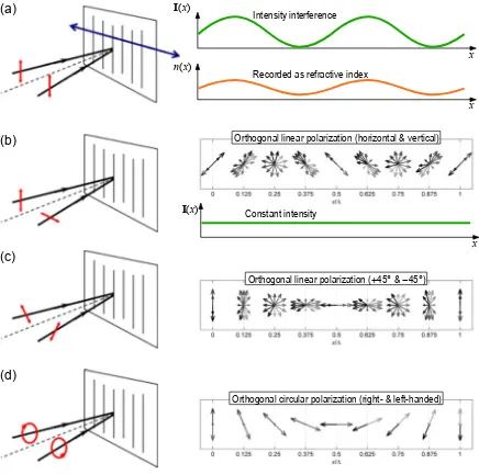
Until now, the most popular approach to create the PG is using polarization holography with organic materials containing azobenzene moieties [12, 13], which can have modest diffraction efficiencies (80%) and a wide range of grating periods[14, 15]. However, it is limited by absorption at visible wavelengths and irreversible degradation when illu-minated or when heated above modest temperatures. An alternative approach employs patterned surfaces which then transfer their anisotropy to a liquid crystal (LC) layer via a photoalignment material [16, 17]. Using this method, we successfully demonstrated defect-free PGs performing their ideal properties [18, 19]. Still, the alignment of liquid crystals remains one of the main fabrication issues and the poor alignment of the LCs causes sig-nificant problems of incoherent scattering, especially when the grating period is relatively small. Substantial experimental studies are considered to optimize the fabrication process for small-period PGs by a careful choice of materials.
The ideal diffraction behavior of the PG was significantly investigated by using the Jones calculus in the paraxial domain [6, 19], where light is treated as a ray making a small angle to the optic axis of the system. The theoretical prediction of PG diffraction properties is no longer valid beyond paraxial approximations (i.e., small grating periods or highly oblique incidence). No work adequately deals with the fundamental question of de-lineating the thin/thick grating regimes in anisotropic gratings. It is, therefore, our desire to investigate PG behavior as the grating period becomes comparable to the wavelength. The study will provide better understanding where the fundamental limits arise and ultimately we seek more practical guidelines for material and processing optimization.
due to two different polarization mechanisms (linear birefringence and optical activity). This unique achromatic diffraction will lead to more diverse utilities of the PG in many photonics applications.
Our aim in this dissertation is to investigate and apply the polarization grating within many areas of photonics and optoelectronic devices. To this end, we first study diffraction behavior of the PG beyond simplistic, limiting assumptions (i.e., paraxial ap-proximation) via numerical modeling of the PGs. We will prove the broadband design of the PG and experimentally demonstrate the achromatic PGs using liquid crystal materials. This dissertation also focuses on the development of three pioneering technologies based on the PG diffraction: (i) Polymer-PG displays; (ii) novel beam steering systems; (iii) advanced spectro-polarimeters. Finally, we expand our exploitation of polarization-based diffractive elements to shape vectorial beam properties. As one of the examples, the ideal Fresnel lens effect by concentric polarization gratings is explored.
In Chapter 2, we start with Maxwell’s equations and then introduce the fundamen-tals of electromagnetic natures of light. Brief descriptions of the polarization of light and different vector representations for polarized light follow. We also discuss light propagation in anisotropic media with optical anisotropy and periodic structures including conventional phase diffraction gratings. A brief summary of material properties of liquid crystals (LCs) and related technologies in optics and photonics is presented. A technical survey of LC diffractive elements for various applications is also given. Chapter 2 is summarized with an introduction of the polarization grating as highly efficient polarizing beam splitters. The theoretical foundations to understand the PG behavior and the fabrication techniques using polarization holography are included.
In the following three Chapters, we discuss our development of technologies based on the PG diffraction. Chapter 4 introduces the polymer-PG display as a viable solution for highly efficient, polarizer-free LCDs. In this Chapter, we show how to achieve polarization-independent modulation using achromatic PGs and conventional LCDs. We also present preliminary results of a prototype of the polymer-PG projection display using a commercial microdisplay and replacing polarizer films with achromatic PGs. Design considerations of the achromatic PGs and techniques for the extinction-ratio enhancement are also discussed. Novel beam steering systems based on the PG diffraction are presented in Chapter 5. We first demonstrated non-mechanical, wide-angle beam steering using stacked LC polarization gratings and waveplates. Several different system designs are considered and the results of a prototype beam steering device are presented. The second beam steering device is the Risley grating, which is a thin-plate version of the Risley prism. This compact beam steering device utilizes a fair of identical PGs that are individually rotated to scan continuous angles within the field of regard. In Chapter 6, we introduce simplified spectropolarimetry using the polarization sensitive diffraction of the PGs and its experimental demonstration at infrared (IR) wavelengths. We also discuss the use of the PGs as polarizing elements for mid-IR spectropolarimeters, especially for astronomical detection. The preliminary experimental results include material feasibility tests of liquid crystals and the PG diffraction properties in mid-IR.
In Chapter 7, the concept and properties of concentric polarization gratings (CPGs) are examined. The CPG is a vectorial version of the Fresnel zone plate that spatially mod-ulate the polarization state of light leading to lens effects. Unlike conventional Fresnel zone plates operating on phase or intensity modulation, the CPGs can exhibit a single diffraction order with sin 100% efficiency in addition to polarization selective lens properties. When a CPG is formed in a liquid crystal cell, an electrically switchable lens can be implemented. In this Chapter, we discuss potential advantages of the CPGs over other Fresnel zone plates (and Fresnel lenses) and also classical volume lenses. We also show preliminary experimental results of CPGs using polarization holography and liquid crystal materials and we summa-rize the Chapter with discussions on potential applications of the CPGs as lens elements or vector (polarization) beam shapers and other possible variations of spatial polarization modulation for generating/manupulating vectorial beam properties.
Chapter 2
Light Propagation in Anisotropic
2.1
Electromagnetic Properties of Lightwaves
The electromagnetic origin of light was significantly understood for the first time by James C. Maxwell [1]. Since his beautiful description of the electromagnetic dynamics, the concealed motion of light is captured by simple mathematical expressions now termed “Maxwell’s equations.” This Section begins with Maxwell’s equations and then introduces electromagnetic properties of lightwaves including polarization of light.
2.1.1 Maxwell’s equations and light propagation
The electromagnetic field can be defined by two vector quantities: the electric and magnetic fields. Maxwell’s equations describe the behavior of these two vector fields in relation to each other and the position and motion of charged particles. In differential form, Maxwell’s equations are given by [22]
∇ ×E(r,t) =−∂B(r,t)
∂t (F araday
"s law) (2.1a)
∇ ×H(r,t) =J(r,t) +∂D(r,t)
∂t (Ampere
"s law) (2.1b)
∇ ·D(r,t) =ρ(r,t) (Gauss"s law) (2.1c)
∇ ·B(r,t) = 0 (Gauss"s law) (2.1d)
wherer is the position vector andt is time. The field variables are defined as:
E:electric f ield(V /m) H:magnetic f ield(A/m)
D:electric displacement(W/m2) B:magnetic f lux density(C/m2)
J:electric current density(A/m2) ρ:electric charge density(C/m3)
These variables (except ρ, a scalar) are vectors and may have complex amplitudes. ρ is a
scalar variable function of space and time.
In order to solve Eq. 2.1, another set of relationships between E (H) and D (B) must be known. These are called constitutive relation [23]. These conditions are established by the physical properties of media; the permittivity εand permeability µ. In a vacuum,
these relations are:
D(r,t) =ε0E(r,t) (2.2a)
where the subscript ‘0’ refers to the value in a vacuum. J can generally be found from Ohm’s law: J(r,t) =σ(r)E(r,t), whereσ is the conductivity. Since materials of interest in
this dissertation are nonmagnetic (at least the effect of magnetic properties is small enough to ignore in normal conditions),µis assumed asµo without any special comment. In linear
media, ε = ε(r) is a function of position. For anisotropic media, permittivity must be
expressed in the form of a tensor ˜ε, which may have different values for each direction of
the electromagnetic field vectors. We will discuss more about material properties and light propagation of anisotropic media in Section 2.2.
Maxwell’s equations in a source-free space, whereσ =ρ= 0, can be rewritten as
∇ ×E(r,t) =−µ∂H(r,t)
∂t (2.3a)
∇ ×H(r,t) =ε∂E(r,t)
∂t (2.3b)
∇ ·E(r,t) = 0 (2.3c)
∇ ·H(r,t) = 0 (2.3d)
The electromagnetic wave equation can be derived from Eqs. 2.3a and 2.3b. We can elimi-nateH by taking the curl of Eq. 2.3a and substituting Eq. 2.3b and we get
∇ ×(∇ ×E) =−µε∂
2E
∂2t (2.4)
Applying the vector identity (∇ × ∇×=∇(∇·)− ∇2) and ∇ ·E= 0, it is reduced to
∇2E− 1
u2
∂2E
∂2t = 0 (2.5)
whereu= (µε)−1/2 is the phase velocity of light propagating in the medium;uin vacuum is given as the special symbolc= (µ0ε0)−1/2 = 2.998×10⁸(m/s), generally called the speed of light. In a dielectric medium, the phase velocity is u=c/n wheren= (ε/ε0)1/2 is referred to as the index of refraction. Without specifying the precise spatial nature of the wave, the time-harmonic electric field can be rewritten as E(r, t) =E(r)ejωt where ω is the angular
frequency. Substituting it into Eq. 2.5, we have
∇2E(r) +k2E(r) = 0 (2.6)
where k = ω/u is the wavenumber and k = ˆkk is defined as the wave vector (ˆk is the
2.1.2 Polarization of light
A uniform plane wave is a particular solution of Maxwell’s equations withE orH assuming the same direction, same magnitude, and same phase in infinite planes perpendic-ular to the direction of propagation (ˆk). While its magnitude, sign and direction can vary in time, the electric field resides in what is known as the plane of vibration. Polarization is the property of an electromagnetic wave or light, which shows the pattern of the electric field vibration. In other words, the polarization of a uniform plane wave describes the locus of the E’s tip at a given point in space as a function of time [3]. Fig. 2.1(a) shows two special cases of polarization states: linear and circular.
An electric field may have only two other components perpendicular to the prop-agation direction. For instance, the electric field vector of lightwave propagating along the
z-axis (ˆk≡zˆ) can be written as follows
E(z, t) = (ˆxEx+ ˆyEy)ej(ωt−kz) (2.7)
whereEx andEy are complex amplitudes ofEcorresponding to ˆxand ˆy, respectively. The
relative difference in magnitude and phase between x- and y-components determines the
polarization state. So it is convenient to rewrite the electric field as
E(z, t) =Ex(ˆx+ ˆyAe−jϕ)ej(ωt−kz) (2.8)
a
b
x
y
ψ
tanχ=±b/a
k k
Linear Polarization Circular Polarization
(a)
(b)
Figure 2.1: Polarization of light: (a) two special polarization states (linear and circular); (b) the polarization ellipse. The polarization state can be described by two characteristic angles of the polarization ellipse: the orientation angle ψ and the ellipticity angle χ as
The magnitudeAand phaseϕallow us to identify three types of polarization states: linear,
circular, and elliptical polarization. Note that A=|Ey/Ex|and ϕ=arg(Ey)−arg(Ex).
The polarization property also can be described by two characteristic angles, re-ferred to as the orientation angle ψ and the ellipticity angle χ of the polarization ellipse. ψ is the angle of the major axis of the ellipse from the +x-axis and χ is determined by
the ratio between the longest diameter ‘a’ and the shortest diameter ‘b’ of the polarization
ellipse as tanχ =±b/a(see Fig. 2.1(b)). Both ψ and χ can be written in terms ofA and ϕby introducing an auxiliary angle α= tan−1A(0≤α≤π/2) as follows
tan 2ψ= 2 tanα
1−tan2αcosϕ (2.9a)
sin 2χ= (sin 2α) sinϕ (2.9b)
Readers may refer to Ref. [3] for more detailed descriptions of the polarization ellipse. For linear polarization states (χ = 0), the locus of E lies on a line oriented at ψ
from the +x-axis. One can say that light has a horizontal linear polarization (HLP) when ψ = nπ and a vertical linear polarization (VLP) when ψ = (n+ 12)π (n is an integer).
For circular polarization states (χ = ±π/4), the polarization ellipse becomes a circle. If χ= +π/4, the electric field vector rotates clockwise and it is so called a right-handed circular
polarization (RCP). Similarly, if χ =−π/4, it is called a left-handed circular polarization
(LCP). Elliptical polarization is the most general type of polarization and, if χ and ψ do
not satisfy the above conditions, light is elliptically polarized.
2.1.3 Jones vector, Stokes parameters, and Poincar´e sphere
The Jones vector is one of the simplest ways to describe polarized light [25]. In 1941 [26], R. Clark Jones invented a simple vector representation for the electric field of a planewave as follows
E=
E0xejϕx
E0yejϕy
= E0ejϕx
cosχ
ejϕsinχ
(2.10)
where E0x,0y and ϕx,y are the instantaneous amplitudes and phase factors for thex and y
components ofE, respectively. E0is the total magnitude of the electric field,E02 =E02x+E02y
and tanχ=E0y/E0x, and ϕ=ϕy−ϕx is the relative phase difference. Light propagation
2×2 matrix that represents the material properties of the medium. This method, often called the Jones matrix analysis orJones calculus, is particularly useful to analyze optical properties of planar/stratified media. The extended Jones matrix method also has been developed for oblique incidence analyses [27]. We note that the Jones vector representation can be applied only to perfectly polarized light. We apply the Jones matrix method to derive analytical expressions for ideal diffraction behavior of a special kind of anisotropic diffraction gratings, known aspolarization gratings.
An important and more general mathematical representation including aspects incoherency for polarized light was developed by G. Stokes in 1852 [28]. He showed that the polarization state of light can be specified by four quantities referred to as the Stokes parameters [3], which are given by
S0=ExEx∗+EyEy∗+EunpolEunpol∗ =E02x+E02y+Iunpol2 (2.11a)
S1=ExEx∗−EyEy∗ =E02x−E02y (2.11b)
S2=ExEy∗+EyEx∗ = 2E0xE0ycosϕ (2.11c)
S2=j%ExEy∗−EyEx∗
&
= 2E0xE0ysinϕ (2.11d)
whereS0 is the total intensity of the light andEunpol is the electric field component
corre-sponding to unpolarized light (Iunpol =|Eunpol|2). S1andS2describe the amount of vertical or horizontal polarization and linear±45◦ polarization, respectively. The last parameterS3 depicts the amount of either right- or left-handed circular polarization depending on its sign (a positive for RHC and a negative for LHC). For fully-polarized light, the Stokes parame-ters satisfy S02=S21+S22+S32 (Iunpol = 0), whileS02≥S12+S22+S32 for partially polarized light. One can determine the degree of polarization P by use of the Stokes parameters as
follows
P = Ipol Itot =
Itot−Iupol
Itot =
'
S2
1+S22+S32
S0 (2.12)
where Ipol is the sum of the intensity of the polarization components and Itot is the total
intensity. It is often convenient to normalize the Stokes parameters by the value of S0 as follows S=
S0" S1" S2" S3"
= 1
Pcos 2χcos 2ψ Pcos 2χsin 2ψ
Psin 2χ
Eq. 2.13 also shows how the Stokes parameters relate to two characteristic angles; the orientation angle (ψ) and the ellipticity angle (χ).
Another useful tool to describe the polarization state of light is the Poincar´e sphere [3], which was developed by Henri Poincar´e in 1892 as a graphical method of de-picting light polarization. The Stokes parameters can be captured in the Poincar´e sphere as shown in Fig.2.2. In particular, the Poincar´e sphere is useful to describe the change in polarized light when it interacts with polarizing elements.
χ !!
!"
!# !$
+%&'( −%&'(
)'(
*'(
+,( ',(
" #
$
ψ
2.2
Light Propagation in Anisotropic and Periodic Media
The vectorial nature of light can lead to different optical properties according to its polarization state when propagation occurs in anisotropic media. In addition, when light travels through/scatters from periodic media, it experiences diffraction or interference, which leads to a spatial modulation of phase or intensity of lightwave. In this Section, we briefly discuss how light interacts with matters while traveling in anisotropic and periodic media.
2.2.1 Light propagation in anisotropic media
Recall the constitutive relation between E and D. For anisotropic media with a directional dependency of the permittivity, a tensor equation is necessary [25]:
D(r,t) =ε0ε˜E(r,t) (2.14) whereε0 is the dielectric constant in a vacuum and a tilde of ˜εsignifies a tensor. One can define an arbitrary permittivity tensor ˜εas follows
˜ ε=
εxx εxy εxz
εyx εyy εyz
εzx εzy εzz
(2.15)
where εmn (m, n =x, y, z) are the normalized permittivities and they could have complex
amplitudes. Note again that we assume non-magnetic material properties (µ=µ0). We first consider a dielectric medium with uniaxial anisotropy in the refractive index only. The permittivity tensor for an arbitrary uniaxial media can be written as
˜
ε=R−1(φ, θ)
εe 0 0
0 εo 0
0 0 εo
R(φ, θ) (2.16)
whereεoandεeare the permittivities for the ordinary and extraordinary waves, respectively.
The indices of refraction for each characteristic waves are defined asno,e=√εo,e. R is the
transformation matrix, which is specified by two angles as follows
R(φ, θ) =
sinφ −cosφ 0
cosθcosφ cosθsinφ −sinθ
sinθcosφ sinθsinφ cosθ
where φ and θ are the azimuthal and polar angles measured from the +x- and +z-axes,
respectively. A difference of the refractive indices ∆nl (= ne−no) is often called linear birefringence of the medium [29]. The normal modes forE corresponding to the ordinary and extraordinary waves can be written as [30]
Eo=
Eox Eoy Eoz = sinφ
−cosφ
0
(2.18a)
Ee=
Eex Eey Eez = n2
ecosθcosφ
n2
ecosθsinφ
−n2osinθ
(2.18b)
Consider linearly polarized light (E = Exxˆ) propagating through a waveplate,
which is a dielectric slab with linear birefringence ∆nl. As the light travels through the
waveplate, it experiences the optical retardation as shown in Fig. 2.3(a). The Stokes
pa-d
(a)
(b)
S1’ S2’
S3’
Δnld/λ(-)
S to ke s P ar am et er s
Figure 2.3: Light propagation in a waveplate: (a) a schematic view of a waveplate (i.e.,
φ = π/4 and ∆nld = λ/4 for a quarter wave retardation); (b) the normalized Stokes
parameters of the output beam as a function of the retardation (∆nld/λ) of the waveplate,
rameters of the emerging light are given by
S1" = cos2(2φ) + sin2(2φ) cos
*2
π∆nld
λ
+
(2.19a)
S2" = cos(2φ) sin(2φ)
, 1−cos
*2
π∆nld
λ
+-(2.19b)
S3" = sin(2φ) sin
*2
π∆nld
λ
+
(2.19c)
whereφ is the orientation of the optic axis of the waveplate,dis the thickness of the slab,
and λ is the wavelength of light (Fig. 2.3(b)). For a simplification, we assume the polar
angleθ= 0. As light travel through the waveplate, it experiences relative phase differences
between two characteristic waves (ordinary and extraordinary) depending on the orientation of the optic axis and the polarization orientation, which is often called retardation. For example, a linear polarization is converted in to a circular polarization whenφ=π/4 and
∆nd=λ/4 (Fig. 2.3)
Certain substances are found to possess the ability to rotate the plane of polariza-tion of light passing through them as illustrated in Fig.2.4(a). This phenomenon is known as
optical activity [2]. Consider a simple medium possessing the following permittivity tensor
˜ ε=
εx −jεg 0
jεg εx 0
0 0 εz
(2.20)
whereεg is the gyration factor. The dispersion relation for a wave propagating along the ˆz
direction is given by
k= ω c
'
εx±εg (2.21)
where the upper sign corresponds to right-handed circular polarization and the lower sign to left-handed circular polarization. Accordingly, the refraction indices for the orthogonal, circular polarizations are
nR='εx+εg (2.22a)
nL='εx−εg (2.22b)
where the subscripts ‘R’ and ‘L’ correspond to the right- and left-handed circular
E
d
(a)
(b)
x y
z
S1’
S2’
S3’
Δncd/λ(-)
S
to
ke
s
P
ar
am
et
er
s
Figure 2.4: Light propagation in an optically active medium: (a) a rotation of the plane of the polarization as light travels in the medium; (b) the normalized Stokes parameters of the output beam as a function of the optical activity (∆ncd/λ).
Consider linearly polarized light (E = Exxˆ) propagating through a slab with
circular birefringence ∆nc. The light experiences the optical rotation as shown in Fig. 2.4(a).
The Stokes parameters of the emerging light are given by
S1" = cos
*2
π∆ncd
λ
+
(2.23a)
S2" =−sin
*2
π∆ncd
λ
+
(2.23b)
S3" =constant= 0, (2.23c)
wheredis the thickness of the slab and λis the wavelength of light (Fig. 2.4(b)). Since the
2.2.2 Light propagation in periodic media
Light propagating through or scattering from periodic structures/surfaces such as gratings experiences diffraction or interference. Conventional diffraction gratings can be classified into two different categories depending on their spatial variations of material properties: phase gratings and amplitude gratings. A phase grating modulates the phase of the propagating wave by its periodically varying refractive index while amplitude grat-ings modulates the amplitude by its absorption coefficient variation. Although there are interesting aspects of the latter case, we limit our discussion to phase gratings and their properties in this Dissertation. We also briefly cover form-birefringent gratings based on subwavelength structures.
Consider two simple examples of phase gratings with sinusoidal and binary index profiles as shown in Fig. 2.5. These gratings are defined by the grating pitch Λ, average index ¯nand index modulation factor n1 as follows
n(x) =
¯
n+n1cos(Gx) for a sinusoidal grating ¯
n+n1{1−22[tan (ftGx)]} for a binary grating
(2.24)
whereGis the grating wave number (2π/Λ), Λ is the grating period, and2(x) is a function
that is 0 outside the interval x = [−1,1] and unity inside it. For binary gratings, the fill
factor ft is a ratio of the area with the higher refractive index (¯n+n1).
The diffraction orders of a grating can be specified by integer numbers known as the Floquet modes (m = 0,±1,±2, . . .). The diffraction angle θm to the mth order is
(a)
(b)
n
n
x
Λ
2
Λ
0
n
n
x
Λ
2
Λ
0
n
1n
1determined by the grating equation [31], defined as follows
sinθm =
mλ
Λ + sinθinc (2.25)
whereθinc is the incident angle.
Most phase gratings can be defined into two different grating regimes depending on their grating parameters (i.e., thickness, period, and refractive index): the Bragg and Raman-Nath regimes. Diffraction characteristics differ for gratings in each regime as shown in Fig. 2.6. It is customary to distinguish among the two regimes of diffraction by defining a dimensionless parameterQ known as theKlein parameter [32, 33]
Q= 2πλd
¯
nΛ2 (2.26)
whered is the grating thickness. In general cases, gratings withQ)1 fall into the Bragg
(or thick) grating regime while gratings with Q < 1 and Λ) λinto the Raman-Nath (or
thin) grating regime. The above descriptions based onQ, however, may be invalid for some
extreme cases such as gratings with too large or too small index contrast. Moharam et al. introduced a new dimensionless parameter ρ[34] defined as follows
ρ= λ
2
¯
nn1Λ2 (2.27)
, which provides more rigorous descriptions of the grating regime. Similar to the case of
Q, the Bragg regime resides in the condition ofρ )1 and the Raman-Nath regime in the
condition ofρ≤1. Note that the grating thickness does not enterρbut it should be chosen
to have reasonable diffraction effect of the grating.
For Bragg gratings (Q)1 or ρ)1), the maximum diffraction occurs where the
incident angle satisfies the following condition
2Λ sinθinc=λ (2.28)
This angle is known as the Bragg angle θB. The diffraction angle of the transmitted wave
is given byθt=θB+ ∆θ, where ∆θrepresents a phase mismatch between the incident and
transmitted waves. The maximum diffraction efficiency of a Bragg grating is given by [25]
ηmax = 1
θ
B!
%
+
&
!
%
+
'
!
%
−
'
!
%
−
&
!
%(
Figure 2.6: The two different grating regimes depending on the grating parameters (i.e., thickness, period, and refractive index): (a) a Bragg or thick grating; (b) a Raman-Nath or thin grating.
whereG is the grating number (2π/Λ) andξ2 is given by (πn
1/λ)2(cosθinccosθt)−1. Note
that the maximum diffraction efficiency can be 100% when ∆θ= 0.
For Raman-Nath gratings (Q * 1 or ρ ≤ 1), a multiple orders may appear in
diffraction as defined in the grating equation (Eq. 2.25). The diffraction efficiencies of sinusoidal phase gratings are given by [25]
ηm =Jm2
* 2
πnd¯ λcosθinc
+
(2.30)
where Jm is themth order Bessel’s function. A binary grating with ft= 12 has diffraction
efficiencies of the mth order as follows
ηm=
cos2ϕ for the 0th order
4(mπ)−2sin2ϕ for themth order
(2.31)
where the phase angle ϕ = πn1d/(λcosθg) and θg is the refractive angle of the grating,
which satisfies ¯nsinθg =n0sinθinc.
Consider a periodic structure composed of subwavelength features of two different media shown in Fig. 2.7 and having permittivity distribution as follows
n(x) =
n1 for (p≤x/Λ≤p+f1)
n2 for (p−f2 ≤x/Λ≤p)
(2.32)
where Λ!λ,p is an integer, andf1+f2 = 1 (f1, f2 >0). The effective dielectric constant
no for the ordinary wave andne for the extraordinary wave are given by
no=
n1n2 '
f1n22+f2n21
(2.33a)
ne=
3
f1n21+f2n22 (2.33b)
and the form-refringence can be defined as ∆n=ne−no. Note that this assembly exhibits
uniaxial anisotropy along the x-axis with a negative birefringence (∆n < 0). One can
modulate the refractive index by varying the thickness of features or rotating the effective optic axis. Extensive studies of subwavelength gratings are found in [36, 37, 38, 39, 40, 41]. Subwavelength gratings are essentially equivalent to anisotropic gratings in naturally birefringent media such as liquid crystals [42, 43, 44].
n
on
en
of
1Λ
f
2Λ
Λ
ε
1ε
22.3
Liquid crystals: soft-condensed matters that control light
Liquid crystal [45, 46, 47] is a phase of soft condensed matter that simultaneously exhibits characteristics of both isotropic liquid and crystalline solids. Since the first dis-covery of cholesteric liquid crystals by Reinitzer in 1888, liquid crystals (LCs) and related technologies have been of great interest to diverse communities in both science and engi-neering. In this Section, we will briefly review several distinct properties of LC materials and their applications in optics and photonics.
2.3.1 Properties of nematic liquid crystal materials
The liquid crystal phases are often characterized by the nature of ordering: posi-tional and orientaposi-tional order. The nematic is one of the most common LC phases that has the lowest degree of ordering with a one dimensional orientation order but no long-range positional order (Fig. 2.8(a)). It is convenient to define a unit vector n, often called the ‘nematic director,’ pointing the average direction of an ensemble of molecules (Fig. 2.8(b)). The deviation from the nematic director n can be quantified with the order parameterS,
E
ε ε
ε
(a)
n
(b)
(c)
splay twist bend
defined asS = 12(3 cos2θ−1) (θis the orientation angle of individual molecules with respect
ton).
The anisotropy in dielectric and optical properties of LCs is a key to enable LCDs and other LC-based electro-optical devices. Consider a nematic LC molecule with the rod-like shape as illustrated in Fig. 2.8(a). The nematic LC exhibits the dielectric anisotropy (expressed as ∆ε=ε%−ε⊥). When an electric fieldEis applied, the field tends to polarize
the free charges within the molecule and leads to a dipole moment. Due to the dielectric anisotropy, this induced dipole moment makes the nematic molecule reorient either parallel (∆ε > 0) or perpendicular (∆ε < 0) to the applied electric field as shown in Fig. 2.8(a).
At optical frequencies, the nematic LC also shows the optical anisotropy, conveniently quantified by a linear birefringence ∆nl = ∆n%−∆n⊥ and light passing through the LC
medium may experience phase retardation (∆nld/λ). The ability of the electro-optic control
of optical anisotropy makes liquid crystals uniquely useful for many applications in optics and photonics. We also note that any static deformation of LCs by external fields and surface interactions can be described by the three basic elastic deformations: splay, twist, and bend (Fig. 2.8(c)).
The elastic continuum theory well explains LC ordering in a finite geometry and applied electric fields [48]. In Ossen-Frank theory, the static free energy densitywf of a LC
volume can be expressed as follows
wf = 12K11[∇ ·n]2+12K22[n· ∇× n]2+12K33[n× ∇ ×n]2 (2.34)
where K11, K22, and K33 are the elastic constants corresponding to the splay, twist, and bend deformations, respectively (Fig. 2.8(c)). Electric fields that are applied across the volume contribute the total energy density by the addition of an extra term: welec =
−12ε0∆ε|E·n|2. Due to chemical and microscopic structural interactions, LCs will typically exhibit a preferred orientation with respect to a surface. This surface influence to LC ordering can be quantified by another extra term: wsurf = 12(wθsin2φ+wφsin2φ) where
wθand wφare surface anchoring strengths (θandφare the polar and azimuth angles of the
nematic director). The equilibrium states for a given set of conditions can be found where the sum w=wf +welec+wsurf is minimized. The resulting configuration of the nematic
director can then be used to find many electro-optical properties.
disser-(c)
Figure 2.9: Types of polymerizable liquid crystal (reactive mesogen or RM) materials: (a) a main-chain LC polymer; (b) a side-chain LC polymer; (c) a chemical structure for a typical RM monomer (RM257 from Merck).
tation. Reactive mesogens (RMs) are liquid crystalline materials with polymerizable end groups [49, 47, 50]. Polymerization of RMs with two or more polymerizable groups leads to densely crosslinked networks in which the liquid crystalline order is permanently fixed. Figs. 2.9(a) and 2.9(b) show two main kinds of reactive mesogens: main-chain and side-chain RMs, respectively. A typical LC diacrylate molecule (RM257 from Merck) is also shown in Fig. 2.9(c). Many interesting applications using these RM materials have been suggested [51, 52, 53, 54, 55, 56, 57, 58]; for example, optical compensation films for LCDs, reflective color filters, and micro-actuators for biomedical applications.
2.3.2 Rubbing techniques of liquid crystal alignment
Although the nematic director is free to point in any direction, LCs typically ex-hibit a preferred orientation with respect to a surface due to chemical and microscopic structural interactions [47]. If the alignment condition is poor (weak anchoring or disconti-nuity), alignment-related defects may appear, such as disclination lines, reverse twist, and reverse tilt. These defects usually lead to considerable light scattering and have large effects on the electro-optical properties of LC devices. It is therefore very important to control the alignment conditions for most LC applications.
Rubbing is the most conventional LC alignment process. When a thin polymer film (i.e., polyimide) is rubbed using a cloth, liquid crystal molecules tend to be aligned by surface interactions. The alignment strength of a uniformly rubbed surface can be quantified by the azimuthal anchoring energywφ (typically,∼10−3J·m−2) defined as follows[59]:
α
Rubbed polymer surface
q A
(a)
Rubbing cloth(b)
Polymer film
Figure 2.10: Rubbing technologies for LC alignment: (a) rubbing of a polymer film; (b) LC alignment by a rubbed polymer surface (groove heightA, pitchq) with a pretilt angle α.
whereK11 is the splay elastic constants of the LC andAand q are the depth (severalµm) and pitch (tens ofµm) of surface relief structures, respectively. The rubbing also generates
a polar directional alignment, called the pretilt angle. Although the polymer rubbing is a simple and effective method for aligning LCs in a large scale, it is often subject to several problems: static charges, non-uniformity, and surface impurities. A number of non-rubbing alignment techniques have been developed, including photoalignment, chemically treated surfaces, and oblique evaporation [60].
2.3.3 Photoalignment of liquid crystal materials
Photoalignment of LCs has become of great interest in display industries due to its capability of the multi-domain alignment for viewing angle improvement of LCDs. The first reports on photoalignment techniques was found in 1988 and 1991 using azobenzene materials [61, 62]. Soon after, in 2002 [16], Schadt and coworkers reported photoalign-ment by dimerization of poly (vinyl cinnamate) photopolymer exposed to linearly polarized UV light, which is known as the linear photo-polymerization (LPP) polymer due to its anisotropic crosslinking selectively responding to linearly polarized light. Although only a few limited types of photoalignment materials were considered in the early development of this alignment techniques, significant improvements have been done during the last decade with more types of photoalignment techniques and increased choices of materials [63, 64, 65]. Applications of photoalignment materials with liquid crystal polymers also successfully draw substantial interests in optical retardation films and color filters.
365nm 440nm trans
cis
(b)
Figure 2.11: Photoalignment of LCs by the photoisomerization of azo-containing polymers: (a) homogeneous to homeotropic transition by a ‘command surface’ treated as aligned azo-dye monolayer (from Ref. [61]); (b) in-plane (or azimuthal) alignment of LCs using the effect of rotation of the azo-dye absorption oscillator (from Ref. [62]).
E
n
LC alignment
(a)
E
(b)
n
α
Figure 2.12: Photoalignment of LCs via linear photopolymerization (LPP): (a) crosslink-ing of polyvinyl 4-methoxy-cinnamate perpendicular the polarization axis (from Ref. [16]); (b) crosslinking of coumarin side-chain polymer parallel to the polarization axis of the il-lumination light. The latter shows a biased tilt angle θ with oblique illumination in the
polarization plane (from Ref. [67]).
involves a molecular axis that actually moves during tis conformation change. A diffusion model of the azo-dye absorption oscillator (chromophore) has been developed to describe this reorientation phenomena [66].
cycloaddition reaction as shown in Fig. 2.12(a). This causes an anisotropic distribution of cyclobutane molecules with their long axis preferably aligned perpendicular to the polar-ization axis and LC alignment also perpendicular to the polarpolar-ization axis. Thus anisotropic Van der Waals interactions of the rigid cores of the anisotropically corsslinked photoprod-ucts are primarily responsible for the alignment of liquid crystals on the LPP surface with two additional factors (anisotropic steric interactions with their partly aligned hydrochar-bon polymer chains and anisotropically depleted prepolymer molecules). In 1996, Schadt et al. reported a modified LPP process based on coumarin side-chain polymers [67]. Similar photo-induced crosslinking can be achieved by the (2+2) cycloaddition reaction as shown in Fig. 2.12(c). There are two very important improvements in comparison with cinna-mate side-chain polymers: (i) coumarin molecules do not give photoisomerization; (ii) the anisotropic crosslinking occurs parallel to the polarization axis and it also leads to LC alignment along the polarization axis. The former removes an issue of alignment stabil-ity in case of the cinnamoyl moiety. The latter shows, for the first time, an azimuthal alignment direction parallel to the electric field of the illumination light. Development of modified LPP photoalignment materials based on endo cinnamic ester polymer molecules and its applications in displays and optical thin films was reported in Ref. [68].
Another important photoalignment mechanism is photodegradation in polyimide materials. The successful photoalignment of a polyimide is considered to be an important technological goal, because of the high thermal stability of polyimides and their acceptance as the alignment layer of choice by the LC display industry. Hasegawa and Taira [69] first reported photoalignment of polyimide by polarized light exposure at 257 nm. Homogeneous LC alignment was obtained in a direction perpendicular to the polarization of the incident UV beam. This is the direction of the maximum density of unbroken polyimide chains on exposure. Therefore, alignment was attributed to the anisotropic depolymerization of the polyimide.
Photoalignment mechanism by anisotropic light desorption was introduced by Nazarenko et al. [70]. This approach may extend the research on photoalignment mate-rials with a great extent from very complex molecular engineering of specialized functional polymers to any possible substrates for liquid crystal devices.
(a)
Rubbed polyimide(b)
Φ
Δφ
Photoaligned layer
Figure 2.13: Anchoring energy of the photoalignment layer: (a) measurement of the az-imuthal anchoring energy using a twisted LC cell with the in-plane sliding mode; (b) the effect of the exposure energy on the anchoring energy. (from Ref. [71])
switching ‘off’ time, the anchoring energy should sufficiently high (e.g., wφ >10−4J/cm2),
comparable with that of the rubbed polymer surface.
Recall the surface anchoring strengths defined as ws = 12(wθsin2φ+wφsin2φ).
The azimuthal anchoring energy wφ can be measured using a Φ-twisted nematic LC cell
assembled with a rubbed polyimide alignment layer on a substrate and a photoalignment layer on the other as shown in Fig. 2.13(a). The value of the apparent twist angle in the LC cell is lower than that the one set by the preferred azimuthal director alignment on the substrates (Φ), because the strong azimuthal anchoring substrate affects the director alignment on the weak azimuthal anchoring one with a photoalignment layer [72]. Assuming the infinite anchoring energy of the rubbed surface, the azimuthal anchoring energy of the photoalignment layer can be calculated from the torque balance equation in the LC cell as follows
wφ=
2K22∆φ
dsin 2(Φ−∆φ) (2.36)
where ∆φ is the measured apparent twist angle. wφ ≈ 10−5 to 10−6J/m2 was reported
from photoalignment layers based on polyvinyl cinnamate derivatives, about one to two orders of magnitude smaller than that of rubbed polyimide layers [73]. Subsequently higher azimuthal anchoring energy wφ > 10−4J/m2, comparable with the anchoring energy of
thinck-ness of the photoalignment layer can strongly affects the alignment quality. For a ultra-thin photoalignment layers, the film may not be uniform or even continuous and the discontinu-ous layer exhibits a lower anchoring energy. However, once a continudiscontinu-ous film is obtained, LC alignment can be achieved with good anchoring properties. Another important factor for the anchoring energy of the photoalignment layers is the exposure energy/dose. Fig. 2.13(b) shows the azimuthal LC anchoring energy of the azo-dye layers depending on the UV dose with varying the exposure time [71].
2.3.4 Liquid crystal applications in displays and photonics
Liquid crystal technology has had a major effect many areas of science and engi-neering, as well as device technology. Applications for this special kind of material are still being discovered and continue to provide effective solutions to many different problems. In this Section, we review three different examples of liquid crystal applications in displays and photonics: (i) flat panel displays, (ii) spatial light modulators, and (iii) diffractive optical elements.
Liquid crystal displays (LCDs) are one of the most popular LC devices with a hugh success of commercialization that utilize distinct electro-optical properties of LC materials. The twisted nematic (TN) LC is the first successful mode of LCDs [75]. Fig. 2.14 illustrates
glass substrates
analyzer color filter
liquid crystal polarizer
(a)
(b)
polarizer analyzer
ON-State OFF-State ITO electrodes
V>Vth
Figure 2.14: Liquid crystal displays: (a) a single pixel of LCDs with a twisted-nematic (TN) LC layer between crossed polarizers (fromhttp://en.wikipedia.org/wiki/Liquid_
the operation principle of TN-LCDs consisting of a 90◦-twisted LC cell sandwiched between
crossed polarizers. In the ‘ON’ state (V = 0), the polarization vector of the incident beam
follows the twist of the liquid crystal directors, which is often called the adiabatic following or waveguiding in the TN-LC. On the other hand, light passes without experiencing waveg-uiding in the ‘OFF’ state (V > Vth) where the LC directors are mostly reoriented normal
to the surface.
There are a number of advantages of LCDs as compared to traditional displays using the cathode ray tube (CRT). Since a LCD is formed in two sandwiched glass substrates with a fewµm gap, the size and weight is dramatically reduced and this flat panel display has
been replacing CRT displays in the last decade. The scalability of LCDs from microdisplays to big screen TVs is another important advantage over even other types of flat panel displays such as plasma displays and digital imaging devices based on MEMS technologies. Even though the LCD technology requires external light sources, it generally shows a low power consumption as compared with that of the CRT. However, some technical challenges remain to improve, including light efficiency, viewing angle, contrast ratio, and response time. While the most advanced LCDs suggest potential solutions for most of these problems, the use of absorbing/reflective polarizers and color filters limit the light efficiency.
LC-based spatial light modulators (SLMs) have become popular to control an op-tical wave-front by altering the phase distribution [76, 77, 78, 79]. A spatial light modulator is a device that imposes some form of spatially-varying modulation (either phase or intensity or both simultaneously) on a beam of light. A typical LC-SLM consists of a liquid-crystal-on-silicon (LCoS) backplane, a LC layer, and a glass substrate coated with a transparent electrode as shown in Fig. 2.15. With combination of the electro-optic control of the LC directors, advanced Si technologies provide a number of attractive characteristics of LC-SLMs such as compactness, high density integration, and low cost. Utilities of LC-LC-SLMs can be found in various photonics applications [80, 81, 79]; for example, holographic data recording, adaptive optical systems, beam steering, optical communication, and projection displays. More recently, holographic optical tweezers have been developed using a high resolution LC-SLMs [82].
Figure 2.15: LC-based spatial light modulator (LC-SLM) (from Boulder Nonlinear Systems, Inc.)
ability to control the director configuration by surfaces and applied fields uniquely makes LC materials attractive to form grating structures with with advanced functions including electro-optical switching/tuning and polarization sensitivity/selectivity.


![Figure 2.18: Liquid crystal grating with the polymer walls (from Ref. [92]): (a) the basicconcept for polarization-independent modulation; (b) the fabrication of the polymer wallvia the polymer diffusion process during selective UV exposure.](https://thumb-us.123doks.com/thumbv2/123dok_us/1253841.1157994/49.612.112.498.375.662/basicconcept-polarization-independent-modulation-fabrication-diusion-selective-exposure.webp)