www.textroad.com
A Review for the Time Integration of Semi-Linear Stiff Problems
Zainal Abdul Aziz1, Nazeeruddin Yaacob2, Mohammadreza Askaripour Lahiji3, Mahdi Ghanbari4
1,2,3
Department of Mathematics, Faculty of Science, Universiti Teknologi Malaysia,81310 UTM Skudai, Johor, Malaysia
4
Department of Mathematics, Islamic Azad University, Khorramabad Branch
ABSTRACT
Several real-world requests that involve conditions where different physical phenomena perform on very different time scales arise simultaneously. The partial differential equations (PDEs) that manage such situations are classified as stiff PDEs. Stiffness is a difficult property of differential equations (DEs) that avoid conservative explicit numerical integrators from managing problem efficiency. There has also been a large compact of importance in the building of exponential integrators. However, different some of the new literature proposes, integrators based on this philosophy have been confirmed since at least 1960.The aim of this study is to review the time integration proposed for semi-linear stiff problems.
KEYWORDS: Exponential methods, numerical inverse Laplace transform, semi-linear parabolic equation.
1. INTRODUCTION
The theory of numerical methods for the time integration of semi-linear stiff problems is well-proposed by the application of exponential methods. Cox and Matthews (2002) studied a clear derivation of the explicit Exact Linear Part (ELP) method, from which they referred the methods as Exponential Time Differencing (ETD) and their implementation of the ETD methods. A modification of the ETD Runge-Kutta schemes of Cox and Matthews has been claimed by Kassman and Terfethen (2005). Maria Lopez-Fernandez (2004) discussed a new algorithm for the implementation of exponential methods ,and the algorithm evaluates the operator by the exponential methods with a quadrature formula that is converges. A spectral order method for inverting sectorial Laplace transforms was studied by Maria Lopez-Fernandez et al. (2006). Moreover, the class of explicit multistep exponential and the explicit exponential Runge-Kutta methods were discussed by Hochbruck and Ostermann (2005).A representation for operators required in the implementation of these integrators in term of suitable Laplace transforms was proposed by Lopez-Fernandez et al. (2005). Other papers on this subject include [1, 4, 5, 7, 10,11,12,13, 14,15,16,17,18,19, 20,21,22, 23, 24, 25].
The problems under consideration can be written as follows:
, (1)
where is a linear operator that represents the highest order of differential terms and is a lower under nonlinear operator. The variation of constants formula is considered for the solution to the initial value problem (1). In Section 2, multistep exponential methods are discussed. In Section 3, exponential Runge-Kutta methods are proposed. In Section 4,evaluationof the mapping required is constructed by the multistep and the Runge-Kutta methods. In Section 5, numerical illustration is presented. Finally, the result is presented.
2. MULTISTEP EXPONENTIAL METHODS
The time integration of problems (1) is demonstrated by a class of explicit exponential methods [16].
with the infinitesimal generator of a -semi group , , of linear bounded operators in
a Banach space [7]. The case of in (1) is sectorial, i.e., is a densely defined and closed linear operator on
and there existsconstants , , and an angle , such that the resolvent fulfils
for . (2)
Then, for , the fractional powers are defined for , and ) endowed
with the graph norm is a Banach space [7]. The nonlinearity in (1) is supposed to be defined on
, for some
for .
The variation of constants formula in interval is presented for step method .
Setting a step size , , and the corresponding time levels ,
, the solution (1) at is given by
. (4)
Given approximations , , after replacing in (4) by the Lagrange interpolation
polynomial of degree , through the points and integrating, the
approximation is obtained.
, (5)
with , ,and the standard forward difference from
, (6)
where
for , , , and are given by
,
(7) ,
The methods considered in (6) are explicit and they require the evaluation .
3. EXPONENTIAL RUNGE-KUTTA METHODS
In the time integration of semi-linear parabolic problems, explicit exponential Runge-Kutta methods have been demonstrated [6, 10].
For , ,and , the approximation to ,with , are presented by
,
(8) ,
with .
The coefficients and are linear combinations of and with
, , , . (9)
Take . The implementing of (8) requires the evaluation of and ,for and
several values of . Besides, the nonlinearity in (1) has satisfied a local Lipchitz condition [16].
4. Evaluation of the vector-valued mapping
Some Laplace transformation formulas are used for getting a suitable representation of the operators ,
, and applied in (6) and (8). For a locally integral mapping , bounded by
, for some , .
For some , , the Laplace transform is noted by
, .
The inverse transform is achieved by means of a suitable rule to discretize the inversion formula ,
where is a contour in the complex plan, running from to and laying in the analytical region of , and it
is noted that [8, 9, 11, 12, 13].
4.1 Evaluation of the mapping required by the multistep methods
,
where, for ,
and . (10)
For every and , the following formula is defined as
. (11)
Thus, for every and ,
. (12)
For
,
and thus the following formula is defined
. (13)
For scalar, the mappings , with are presented by
, ,
(14)
, .
In order to evaluate , , the formulas (14) with instead of are proposed.For
approximating the original mapping at the inversion of the Laplace transform has been performed [8, 9].
In this way, the following formulas are invert of Laplace transforms that we need: ,
,
(15) ,
,
.
Note that because of (2), the mapping turns out to be sectorial in the variable , i.e., there exists
constants and , possibly different form of the constants in (2), such that
is analytic for in the sector and there
, for some . (16)
The formulas in (15) can also be considered by combining the Cauchy integral formula [7, 8, 14] with the inversion formula for Laplace transform. For suitable contours and in the complex plan, both of them lay the resolvent set of ,whichholds
(17)
.
4.2 Evaluation of the mapping by the Runge-Kutta methods
For in (9), and ,the following formula is considered [8, 9,15]
,
where for , ,
, (19)
and . Then, for every and ,
. (20)
The same as argument in (17) justifies the operators and , , , which can be
calculated by applying the inversion of the Laplace transforms
, , , , (21)
to approximate the original mapping at [8].
5. Numerical illustration
In this part, the same examples are proposed [6, 16].
5.1 Example for the multistep exponential methods
The following problem is demonstrated [16]
, (22)
for and , subject to homogeneous Dirichlet boundary conditions and with such that the
exact solution to (22) is . Moreover, in the example, the mapping
, (23)
is considered [8].
Table 1: in (23) for is computed,and the absolute error obtained is displayed by
MATLAB with and .
In the table, the spatial discretization of (22) is implemented by applying standard finite differences with
spatial nodes, centered for the approximation of .
The nonlocal term has been presented by the composite Simpson’s formula [16]. Moreover, the formula (6) is
utilised with , for integrating in time the semi discrete problem so that is
matrix
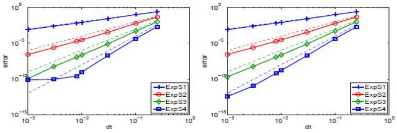
Figure 1: Error of exponential multistep methods (6) utilised to (22), for , and 4. Left:
With quadrature nodes on the hyperbolas, Right: With .
In Figure 1, the error versus the step size at is shown and measured in a discrete version of the norm
, for and . In Figure 1 also, lines of slope 1, 2, 3, and 4 are observed to visualise the order
of convergence [16]. In fact, it is higher than the one predicted in [16].
5.2Example of the exponential Runge-Kutta methods
In this section, two examples are proposed [6]. The first following problem is considered [6]
, (24)
for and , subject to homogeneous Dirichlet boundary conditions and with such that the
exact solution to (24) is . Moreover, the Butcher tableaus are applied with the
abbreviations
, and , .
This problem is discretised in space by standard finite differences with grid points. For the time
integration of semidiscrete problem, the equations (8) are considered with
, and the second order method
(25)
the third-order method
(26) and the fourth-order method
and
In the implementation of the second order method, to invert four different Laplace transforms, the form of (21)
is needed for approximating , , , and . In addition, the inversion of eight Laplace
transforms is required in the implementation of the third-order and fourth-order methods.
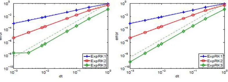
Figure 2: Error of Runge-Kutta methods (8) with (25), (26), and (27) utilized to (24). Left: With quadrature nodes, Right: .
In Figure 2, the error at versus the step size is displayed and measured in the maximum norm. In
order to test the algorithm, lines with the corresponding slopes in Figure 2 are added. For this kind of methods,
full precision for are seen [6].
The second following problem is presented [6]
, (28)
for and , subject to homogeneous Dirichlet boundary conditions and with such that the
exact solution to (28) is .
This problem in space is discretized as in the previous example (22), and the composite Simpson’s rule is applied for the approximation of the nonlocal term. For the time integration, the formulas (8) are used with
, (25), and (26).
Figure 3: Error of Runge-Kutta methods (8) with , (25), and (26) applied to (28). Left: With quadrature nodes, Right: With .
In Figure 3, the error at is shown and measured in a discrete version of the norm [6]. The
order of convergence for this problem is expected, where the first order is 1, 1.75 for (25), and 2.75 for (26). Lines with the corresponding slopes in Figure 3 are added in order to check the algorithm for exponential
6. Conclusions
In this work, the way to approximate the exponential operators required for the implementation of different kinds of exponential methods has been derived, which have been demonstrated for the time integration of semi-linear problems. Moreover, the numerical inversion of the Laplace transform and its applications have been shown. Two examples of the multistep exponential and the exponential Runge-Kutta methods have also been considered.
REFERENCES
[1] H. Berland, B. Skaestad, and W. M. Wright. EXPINT - A Matlab Package for Exponential Integrators. ACM Transactions on Mathematical Software, 33:Article Number 4, 2007.
[2] S. M. Cox and P. C. Matthews, Exponential time differencing for stiff systems, J. Comput. Phys., 176, 430– 455, 2002.
[3] A. K. Kassam. High Order Time stepping for Stiff Semi-Linear Partial Differential Equations. PhD thesis, Oxford University, 2004.
[4] A.-K. Kassam and L. N. Trefethen, Fourth-order time stepping for stiff PDEs, SIAM J. Sci. Comp., 26, 1214–1233, 2005.
[5] M. Hochbruck, A. Ostermann, Exponential Runge–Kutta methods for parabolic problems, Appl. Numer.
Math. 53, Issues 2-4, 323-339, 2005.
[6] M. Hochbruck, A. Ostermann, Explicit exponential Runge–Kutta methodsfor semi linear parabolic
problems, SIAM J. Numer. Anal. 43, No. 3, 1069-1090, 2005.
[7] D. Henry, Geometric theory of semi linear parabolic equations. Lecture Notes in Mathematics 840, Springer, Berlin, 1981.
[8] M. L´opez- Fern´andez, C. Palencia, A. Sch dle, A spectral order method for inverting sectorial Laplace
transforms, SIAM J. Numer. Anal., 44, pp.1332– 1350, 2006.
[9] M. L´opez- Fern´andez, C. Palencia, On the numerical inversion of the Laplace transform of certain
holomorphic mappings, Appl. Numer. Math., 51,pp. 289–303, 2004.
[10] M. L´opez- Fern´andez, C. Lubich, C. Palencia, A. Schadle, Fast Runge-Kutta approximation of
inhomogeneous parabolic equations, Numer. Math., 102, pp. 277–291, 2005.
[11] J. A. C. Weideman, L. N. Trefethen, Parabolic and hyperbolic contours for computing the Bromwich
integral, Math. Comput. 76, pp. 1341–1356, 2007.
[12] I. P. Gavrilyuk, W. Hackbusch, B. N. Khoromskij, Data-sparse approximation to a class of
operator-valued functions, Math. Comp., 74, pp. 681–708, 2005.
[13] D. Sheen, I. H. Sloan, V. Thom´ee, A parallel method for time discretization of parabolic equations based
on Laplace transformation and quadrature, Math. Comp., 69, pp. 177–195, 2000.
[14] G. H. Golub and C. F. Van Loan. Matrix Computations. The Johns Hopkins University Press, Baltimore, MD, third edition, 1996.
[15] M. L´opez-Fern´andez, On the implementation of exponential methods for semi- linear parabolic equations, arXiv. math.NA, 2008.
[16] M. P. Calvo, C. Palencia, A class of explicit multistep exponential integrators for semi-linear problems, Numer. Math. 102, pp. 367–381, 2006.
[17] J. D. Lawson. Generalized Runge-Kutta Processes for Stable Systems with Large Lipschitz Constants. SIAM J. Numer Anal., 4:372-380, 1967.
[18] B. V. Minchev and W. M. Wright. A Review of Exponential Integrators for First Order Semi-Linear Problems. Tech. Rep. NTNU, Preprint. 2005.
[19] J. Certaine. The Solution of Ordinary Differential Equations with Large Time Constants. In Mathematical Methods for Digital Computers, A. Ralston and H. S. Wilf, eds.:128-132, Wiley, New York, 1960.
on Laplace transformation and quadrature, Math. Comp., 69 , pp. 177–195, 2000.
[22] L. F. Shampine and C. W. Gear. A User's View of Solving Stiff Ordinary Differential Equations. SIAM Review, 21:1-17, 1979.
[23] Q. Nie, Y.-T. Zhang and R. Zhao, Efficient semi-implicit schemes for stiff systems, Journal of Computational Physics, 214 , 521-537. 2006.
[24] G. Beylkin and J. M. Keiser, On the adaptive numerical solution of nonlinear partial differential equations in wavelet bases, J. Comput. Phys., 132 ,233–259, 1997.