An Adaptive Grid Algorithm for Air Quality Modeling

(1)

SRIVASTAVA, RAVI K. An Adaptive Grid Algorithm for Air Quality Modeling. (Under the direction of Dr. D. Scott McRae.)

The physical and chemical processes responsible for air pollution span a wide range of spatial scales. For example, there may be point sources, such as power plants that are characterized by relatively small spatial scales compared to the size of the region that may be impacted by such sources. To obtain accurate distributions of pollutants in an air quality simulation, the pertinent spatial scales can be resolved by varying the physical grid node spacing.

A new dynamic adaptive grid algorithm, the Dynamic Solution Adaptive Grid

Algorithm - PPM (DSAGA-PPM), is developed for use in air quality modeling. Given a

fixed number of grid nodes, DSAGA-PPM distributes these nodes in response to spatial resolution requirements of the solution field and then updates the solution field based on the resulting distribution of nodes. DSAGA-PPM is implemented dynamically to resolve any evolving solution features.

(2)

mean-square errors in DSAGA-PPM results are about 4-5 times lower than those in the corresponding SGA-PPM results.

Tests with reacting species and sources demonstrate that DSAGA-PPM provides the needed solution resolution. In simulations of a rotating and reacting conical puff, the root-mean-square errors in DSAGA-PPM results are about 4-6 times lower than those in the corresponding SGA-PPM results. In simulations of a power plant plume, the

DSAGA-PPM solution reflects the early, the intermediate, and the mature stages of plume development; these stages are not seen in the corresponding SGA-PPM solution. Finally, it is demonstrated that DSAGA-PPM provides an accurate description of the ozone production resulting due to dynamic interactions between emissions from two power plants and an urban area. In general, these results reflect that DSAGA-PPM is able to provide accurate spatial and temporal resolution of rapidly changing and complex concentration fields.

(3)

(4)

DEDICATION

In memory of my father: Krishna Kant Srivastava

(5)

BIOGRAPHY

Ravi K. Srivastava was born in Varanasi, India, on March 26, 1955. After graduating from Methodist High School in 1974, he attended Indian Institute of

Technology, Kanpur (IIT Kanpur). Ravi received a Bachelor of Science in Mechanical Engineering from IIT Kanpur in 1979. From 1979 to 1982, Ravi worked with several companies in India including Larsen & Toubro Ltd., Perfect Machine Tools Co., and Crompton and Greaves Ltd. In September 1982, he began graduate study at Washington State University (WSU). Ravi received his Master of Science in Mechanical Engineering from WSU in December 1984. From 1985 through 1994, he worked as a combustion engineer with Acurex Environmental Corporation. During this period, Ravi published numerous papers on air pollution control and coinvented a sorbent injection process designed to control combustion generated metal aerosol. For this process, Ravi and other coinventors obtained a U.S. patent. In 1989, he entered in the Ph.D. program in

aerospace engineering at North Carolina State University. Since 1994, Ravi is employed with the Acid Rain Division of the U.S. Environmental Protection Agency in

(6)

ACKNOWLEDGEMENTS

I would like to acknowledge and thank everyone who made the completion of this dissertation possible. I would especially like to thank my advisor, Professor D. Scott McRae, for his encouragement, guidance, and patience through the years. My

appreciation and thanks to Dr. M. Talat Odman for his numerous helpful insights and suggestions that guided the development of this dissertation. Thanks also to Dr. F.R. DeJarnette and Dr. R.E. White, my other committee members. Many thanks to Mr. Larry Kertcher, my supervisor, for allowing me time away from work at critical junctures.

Finally, I would like to thank my family and friends who have been a constant source of support for me through the years of this research. I especially thank my wife Jenny, my daughter Katie, and my mother Kusum for their patience, love, and

encouragement. Thanks are also extended to Mr. Dominic Mancini and Mr. Peter Tsirigotis for providing me patient ears every now and then.

(7)

List of Tables

2.1 Some Generalized Vertical Coordinates ... ..26

4.1 Values of Adaptation Parameters Used in One-Dimensional Tests... ..70

4.2 Error Characteristics for the One-Dimensional Tests ... ..71

4.3 Error Characteristics for the Simulations of a Rotating Cone... ..82

4.4 Error Characteristics for the Simulations of Multiple Rotating Cones ... ..88

6.1 A Simplified Chemical Mechanism for Photochemical Production of Ozone... ..99

6.2 Initial Concentrations of Species in the Pollutant Puff ... 101

6.3 EVALLEY and EPEAK for the 150 Seconds Simulation of the Puff... 120

6.4 EMAS, EVAR, and ERMS for the 150 Seconds Simulation of the Puff... 120

6.5 EVALLEY and EPEAK for the 86,400 Seconds Simulation of the Puff... 134

6.6 EMAS, EVAR, and ERMS for the 86,400 Seconds Simulation of the Puff ... 134

7.1 Initial Concentrations and Source Terms for the Power Plant Plume Model Problem ... 139

8.1 VOC and NOx Initial Concentrations and Source Terms for the Multiple Sources Model Problem ... 162

8.2 Cell Volumes in the Vicinity of the Downwind Point Source ... 176

8.3 O3 Metrics for Each of the Simulation Results ... 193

9.1 CPU Times Associated With Rotating Cone Simulations ... 196

9.2 CPU Times Associated With Simulations of Multiple Sources... 198

(10)

List of Figures

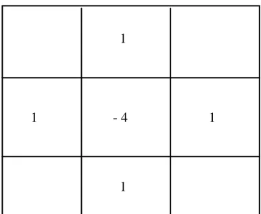
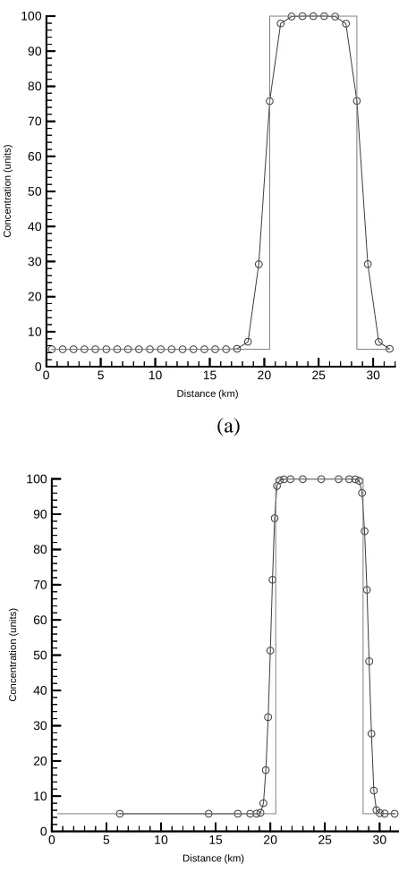
2.1 Tangential Cartesian Coordinates ... ..23 2.2 Spherical Coordinates... ..24 3.1 The five-point stencil for computing discretized Laplacian... ..57 3.2 Grid node o and neighboring cells used in the center-of-mass scheme... ..60 4.1 Rectangular waveform solution obtained with (a) SGA-PPM

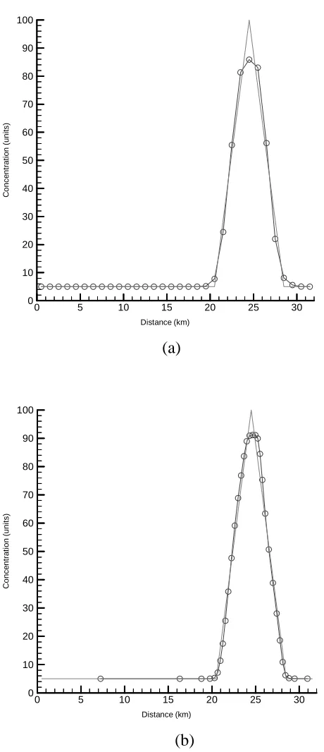
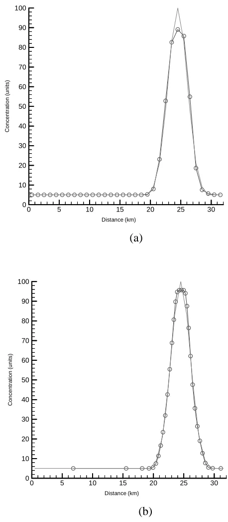
(b) DSAGA-PPM ... ..73 4.2 Triangular waveform solution obtained with (a) SGA-PPM

(b) DSAGA-PPM ... ..74 4.3 Gausian waveform solution obtained with (a) SGA-PPM

(b) DSAGA-PPM ... ..75 4.4 Preadapted grid showing clustering of nodes near the cone... ..78 4.5 Solution field (a) with oscillations (b) without oscillations ... ..79 4.6 Rotating cone results obtained with (a) SGA-PPM

(b) DSAGA-PPM ... ..80 4.7 Adaptive grid after one revolution of the cone... ..81 4.8 Preadapted grid showing clustering of nodes near the cones... ..84 4.9 Results for four cones obtained with (a) SGA-PPM

(b) DSAGA-PPM ... ..86 4.10 Adaptive grid after one revolution of the cones ... ..87 4.11 DSAGA-PPM solution obtained using a refined grid

with 85 x 85 nodes ... ..89 4.12 Adaptive refined (85 x 85 nodes) grid after one revolution

(11)

6.1 Changes in concentrations of selected species over 150 seconds

(a) peak concentrations (b) background concentrations... 103 6.2 Changes in concentrations of selected species over 86,400 seconds

(a) peak concentrations (b) background concentrations... 104 6.3 Preadapted grid reflecting clustering of nodes in and around

the pollutant puff ... 106 6.4 NO distribution after 150 seconds in the pollutant puff

(a) exact solution on uniform grid (b) SGA-PPM solution ... 108 6.5 NO distribution after 150 seconds in the pollutant puff

(a) exact solution on adaptive grid (b) DSAGA solution... 109 6.6 NO2 distribution after 150 seconds in the pollutant puff

(a) exact solution on uniform grid (b) SGA-PPM solution ... 110 6.7 NO2 distribution after 150 seconds in the pollutant puff

(a) exact solution on adaptive grid (b) DSAGA solution... 111 6.8 O3 distribution after 150 seconds in the pollutant puff

(a) exact solution on uniform grid (b) SGA-PPM solution ... 112 6.9 O3 distribution after 150 seconds in the pollutant puff

(a) exact solution on adaptive grid (b) DSAGA solution... 113 6.10 HCHO distribution after 150 seconds in the pollutant puff

(a) exact solution on uniform grid (b) SGA-PPM solution ... 114 6.11 HCHO distribution after 150 seconds in the pollutant puff

(a) exact solution on adaptive grid (b) DSAGA solution... 115 6.12 Adaptive grid after 150 seconds reflecting clustering of nodes

in and around the pollutant puff ... 116 6.13 NO distribution after 86,400 seconds in the pollutant puff

(a) exact solution on uniform grid (b) SGA-PPM solution ... 123 6.14 NO distribution after 86,400 seconds in the pollutant puff

(12)

6.15 NO2 distribution after 86,400 seconds in the pollutant puff

(a) exact solution on uniform grid (b) SGA-PPM solution ... 125

6.16 NO2 distribution after 86,400 seconds in the pollutant puff (a) exact solution on adaptive grid (b) DSAGA-PPM solution... 126

6.17 O3 distribution after 86,400 seconds in the pollutant puff (a) exact solution on uniform grid (b) SGA-PPM solution ... 127

6.18 O3 distribution after 86,400 seconds in the pollutant puff (a) exact solution on adaptive grid (b) DSAGA-PPM solution... 128

6.19 HCHO distribution after 86,400 seconds in the pollutant puff (a) exact solution on uniform grid (b) SGA-PPM solution ... 129

6.20 HCHO distribution after 86,400 seconds in the pollutant puff (a) exact solution on adaptive grid (b) DASGA-PPM solution... 130

6.21 Adaptive grid after 86,400 seconds reflecting clustering of nodes in and around the pollutant puff... 131

7.1 Preadapted grid reflecting clustering of nodes near the point source... 140

7.2 SGA-PPM prediction of NO concentration after 40,000 seconds... 142

7.3 DSAGA-PPM prediction of NO concentration after 40,000 seconds... 142

7.4 SGA-PPM prediction of O3 concentration after 40,000 seconds ... 143

7.5 DSAGA-PPM prediction of O3 concentration after 40,000 seconds ... 143

7.6 Three-dimensional depiction of SGA-PPM results for O3 concentration at 40,000 seconds... 144

7.7 Three-dimensional depiction of DSAGA-PPM results for O3 concentration at 40,000 seconds... 144

(13)

7.8(b) SGA-PPM and DSAGA-PPM predictions of O3 concentration

in plume cross-section at a distance of (b) 30 km downwind of

the source. SGA concentrations are depicted by the dotted curve ... 148

7.8(c) SGA-PPM and DSAGA-PPM predictions of O3 concentration in plume cross-section at a distance of 135 km downwind of the source. SGA concentrations are depicted by the dotted curve ... 149

7.9 DSAGA-PPM prediction of O3 concentration field at 3600 seconds ... 151

7.10 DSAGA-PPM prediction of O3 concentration field at 10,800 seconds .. 151

7.11 Adaptive grid after 40,000 seconds reflecting clustering of nodes near the source and in the plume ... 152

7.12 Refined grid SGA-PPM prediction of O3 concentration field at 40,000 seconds ... 155

7.13(a) Refined grid SGA-PPM and DSAGA-PPM predictions of O3 concentration in plume cross-section at a distance of 10 km downwind of the source. Refined grid SGA concentrations are depicted by the dotted curve... 156

7.13(b) Refined grid SGA-PPM and DSAGA-PPM predictions of O3 concentration in plume cross-section at a distance of 30 km downwind of the source. Refined grid SGA concentrations are depicted by the dotted curve... 157

7.13(c) Refined grid SGA-PPM and DSAGA-PPM predictions of O3 concentration in plume cross-section at a distance of 135 km downwind of the source. Refined grid SGA concentrations are depicted by the dotted curve... 158

8.1 Preadapted grid reflecting clustering of nodes near the point sources and in and around the urban area source... 165

8.2 SGA-PPM prediction of NO concentration after 40,000 seconds... 166

8.3 DSAGA-PPM prediction of NO concentration after 40,000 seconds... 166

(14)

8.5 DSAGA-PPM prediction of O3 concentration after 40,000 seconds ... 167

8.6 Three - dimensional depiction of the O3 concentration field resulting from the SGA-PPM simulation for 40,000 seconds... 168

8.7 Three - dimensional depiction of the O3 concentration field resulting from the DSAGA-PPM simulation for 40,000 seconds ... 168

8.8 Adaptive grid after 40,000 seconds reflecting clustering of nodes around the upwind point source and in and around the urban area... 172

8.9(a) OH weight function at 40,000 seconds ... 173

8.9(b) HO2 weight function at 40,000 seconds ... 173

8.9(c) O3 weight function at 40,000 seconds ... 174

8.9(d) Final smoothed weight function at 40,000 seconds ... 174

8.10 SGA-PPM prediction of O3 concentration field at 40,000 seconds in simulation without the upwind point source ... 177

8.11 DSAGA-PPM prediction of O3 concentration field at 40,000 seconds in simulation without the upwind point source ... 177

8.12 DSAGA-PPM prediction of NO concentration field at 3,600 seconds ... 179

8.13 DSAGA-PPM prediction of OH concentration field at 3,600 seconds ... 179

8.14 DSAGA-PPM prediction of HO2 concentration field at 3,600 seconds ... 180

8.15 DSAGA-PPM prediction of O3 concentration field at 3,600 seconds ... 180

8.16 Adaptive grid at 3,600 seconds reflecting clustering of nodes at the point sources and in and around the urban area... 183

(15)

8.18 DSAGA-PPM prediction of OH concentration field at

25,200 seconds ... 184 8.19 DSAGA-PPM prediction of HO2 concentration field at

25,200 seconds ... 185 8.20 DSAGA-PPM prediction of O3 concentration field at

25,200 seconds ... 185 8.21 Adaptive grid at 25,200 seconds reflecting clustering of nodes

around the upwind point source and in and around the urban area... 187 8.22 DSAGA-PPM prediction of NO concentration field at

39,600 seconds ... 189 8.23 DSAGA-PPM prediction of OH concentration field at

39,600 seconds ... 189 8.24 DSAGA-PPM prediction of HO2 concentration field at

39,600 seconds ... 190 8.25 DSAGA-PPM prediction of O3 concentration field at

39,600 seconds ... 190 8.26 Adaptive grid at 39,600 seconds reflecting clustering of nodes

around the upwind point source and in and around the urban area... 191 8.27 Refined grid SGA-PPM prediction of NO concentration field at

40,000 seconds ... 194 8.28 Refined grid SGA-PPM prediction of O3 concentration field at

(16)

List of Symbols

Uppercase

A, B, and C coordinate systems in E3

A_b base area of a three dimensional cell

D_l molecular diffusivity of species l

E3 the Euclidean space

E, F, G mass fluxes in x, y, and z directions, respectively

E_lP X t

P

( r , ) mass emission rate of the point source located at Xr_P

El A

mass emission flux from an area source

H x y t( , , ) top of the modeling domain in Cartesian space

J Jacobian of transformation

K, Kmn symmetric turbulent diffusivity tensor, m = 1, 2, 3

and n = 1, 2, 3

K_xx, K_yy horizontal turbulent diffusivity components

Kzz vertical turbulent diffusivity

L three-dimensional, semi-linear differential operator

M number of interim steps

Ml molecular weight of species l

N number of species

(17)

r

P_i the position coordinates in physical space of the centers of the cells that are local to the grid node o; i =1,...,4.

Rl net generation of chemical species l by chemical reactions

Rs stiffness ratio

ℜ Universal gas constant

S_l rate of source addition for the chemical species l

S_lP rate of change of concentration due to point source

S_lA

rate of change of concentration due to area source

T temperature of air

V cell volume in physical space

r r

V X t( , ) wind field in Ω( )t

Vl g

pollutant deposition velocity

r

X position vector in Ω( )t

r

X₁, Xr₂ physical locations in Cartesian coordinates

Lowercase

a (X , t), b (r X , t)r coefficients associated with boundary conditions

cl concentration of l

th

species

c_{l in}, c_{l out} species concentrations at inflow and outflow boundaries,

respectively

(18)

e1, e2 volume weighting parameters

gi j the metric tensor for the coordinate system x m

g_l (X , t)r species specific boundary condition coefficient

h t( ) mixing layer height

r r r

i j k, , unit vectors along x, y, z directions, respectively

kj temperature dependent rate constant for j

th

reaction r

n the unit outward normal vector to bounding surface dS r

nH,

r

nT unit normals to the horizontal boundary and the top surface

of the modeled domain, respectively

p pressure

q_l mass mixing ratio for species l

rj the reaction rates of the m individual reactions, j = 1,...,m

t time

u, v, w velocity vector components along x, y, z directions,

respectively r

uH,

r

uT advective velocity in the horizontal plane and with respect

to the top surface of the modeled domain, respectively $

uboundary velocity at the boundary

vm contravariant velocity components in xm_. r

v_b velocity of an element of the bounding surface dS

(19)

wmin minimum allowable weight function

x Cartesian coordinate system

x_t, y_t_,z_t tangential Cartesian coordinates

xm

a coordinate system (x1, x2, x3)

xα a coordinate system (x1, x2, x3, x4 = t)

x, y, z Cartesian space vector components

Greek

α αk, o _{coefficients defining discrete Laplacian}

α βjl, jl the reactant and the product stoichiometry, respectively, in

the reaction step j; j = 1,...,m

β

m interim step iteration count

ρ _{density of air}

γ _{determinant of metric tensor}

θ solar zenith angle

λ

l eigenvalues of the Jacobian Matrix

J R

c l N j N

c l j

= ∂_∂ ; =1,..., ; =1,..., .

Ψ any property (e.g., concentration)

Ω( )t time varying, spatial region

ΩCV

(20)

∂ Ω( )t boundary surface of Ω( )t

δt a time period

ξ η ζ, , general curvilinear coordinates

σ direction normal to ∂ Ω( )t .

∆ t basic time step of atmospheric diffusion equation

∆Xr_{i j}_, change in position coordinates of the node i, j

∆ ξ, ∆ η cell spacing in ξ and η directions, respectively

∆2

discrete approximation of Laplacian

Subscripts and Superscripts

adv pertaining to advection

c pertaining to chemistry

diff pertaining to diffusion

e exact or reference

g grid time

i, j, k array positions, values associated with grid cell

l species index, l = 1,...,N

min, max minimum and maximum values

n, (n+1), n+1 time level indicators

(21)

o grid node o

p values associated with cell side

s pertaining to source terms

x, y, z, t partial derivatives with respect to given Cartesian variable

ξ η ζ, , partial derivatives with respect to given transformation

space variable

Accents

− denotes Reynolds averaged or cell averaged value

∧ denotes a transformed quantity

denotes an ensemble averaged quantity

) denotes cell side sweep volume-averaged value

Abbreviations / Chemical Names

AQM air quality model

CFL Courant-Friedrichs-Levy number

CIE Conservative Interpolation Equation

CO carbon monoxide

CO2 carbon dioxide

DSAGA Dynamic Solution Adaptive Grid Algorithm

HC lumped hydrocarbons

(22)

HNO3 nitric acid

H2O water

HO2 hydroperoxyl radical

Mflops million floating point operations per second

NO nitric oxide

NO2 nitrogen dioxide

NOx nitrogen oxides

OH hydroxyl radical

O3 ozone

ppb parts per billion

PPM Piecewise Parabolic Method

ppmv parts per million by volume

rad radians

RMS root-mean-square

RO2 alkylperoxy radical

SIERRA Solver Independent, Efficient r-Refinement Algorithm

(23)

It is quite a three-pipe problem.

(24)

One of the major concerns facing the world currently is the impact of

anthropogenic activities on the environment. Detrimental impacts on the environment resulting from acid deposition; increase in concentrations of greenhouse gases, fine particles, and tropospheric ozone (O3); and depletion of stratospheric O3 have been the

focus of many research and regulatory activities. Over the next two decades, many far-reaching policy decisions will have to be made to address these impacts. Since these decisions will have a direct bearing on our health and lifestyle, it is imperative that research programs continue to provide, or improve, the scientific foundations for these decisions.

(25)

Numerical simulations conducted using air quality models (AQMs) are used to determine the impacts of air pollution on the environment. Specifically, the predictions of AQMs are used in establishing ambient air quality standards aimed at protecting public health with an adequate margin of safety. Additionally, AQM predictions are also used to develop effective emission reduction strategies focussed on attainment of ambient air quality standards. Since the predictions of AQMs have, and will continue to have, a direct bearing on public health and lifestyle, it is quite important that efforts continue to be made to improve the accuracy of these predictions.

The physical and chemical processes responsible for air pollution span a wide range of spatial scales. For example, there may be point sources, such as power plants, that are characterized by relatively small spatial scales compared to regional-scale pollutant plumes from such sources. Therefore, in order to accurately model transport and chemistry of air pollutants, an AQM has to be able to adequately resolve the pertinent spatial scales. This can be achieved by varying the physical grid node spacing in an AQM to provide resolution where needed.

(26)

inability to adjust to dynamic changes in solution resolution requirements. Another approach to achieving local solution resolution involves using dynamic adaptive grids. In principle, such grids would be continuous and would dynamically adjust to changing solution resolution requirements. Therefore, use of such grids would not be constrained by the limitations associated with use of nested grids.

Recently, ideas promoting use of dynamic adaptive grids in atmospheric modeling are gaining in popularity. Dietachmayer and Droegemeier [3] use a variational formulation of adaptive grid generation equations to compute solutions to test problems. Almgren et al. [4] have used a nested hierarchy of grids, with simultaneous refinement of grids in both space and time, to compute the release of hot gas into the atmosphere. Skamarock and Klemp [5] have used a hierarchical grid approach to model a compressible formulation of atmospheric flow equations. Recently, Tomlin et al. [6] have investigated the use of an adaptive unstructured grid method to obtain solutions of test problems of interest in air quality modeling.

A grid adaptation algorithm suitable for use in aerospace applications has been developed by Benson and McRae [7-9]. This algorithm, called the Dynamic Solution

Adaptive Grid Algorithm (DSAGA), uses weight functions constructed from absolute

(27)

are corrected. This correction is completed using an equation obtained by splitting the time-dependent terms from the steady terms in the general conservation laws for moving control volumes. DSAGA has been used to compute unsteady, three-dimensional, turbulent, viscous flows [10-12]. Additionally, Srivastava et al. [13] have used DSAGA to compute test cases of interest in air quality modeling. Recently, Laflin and McRae [14] and Laflin [15] have developed the Solver-Independent, Efficient r-Refinement

Algorithm (SIERRA) that provides robust and computationally efficient implementation

strategies for grid adaptation algorithms. SIERRA incorporates a solver-independent weight function and a solver-independent solution field redistribution procedure.

Developed in this work is a new dynamic adaptive grid algorithm that is suitable for use in AQMs. This algorithm was built on the foundation provided by the DSAGA algorithm of Benson and McRae [7-9]. However, the new algorithm extends the DSAGA framework by utilizing more accurate solution procedures. Specifically, the new algorithm uses the Piecewise Parabolic Method (PPM) developed by Collela et al. [16] for computing the advective fluxes and the fluxes resulting from grid movement. Moreover, the new algorithm incorporates the SIERRA weight function and solution field redistribution procedure. This new algorithm is called the Dynamic Solution Adaptive

Grid Algorithm - PPM (DSAGA-PPM). The subsequent chapters describe the

(28)

Using tensor calculus, the governing equations for the current Eulerian air quality models are derived in Chapter 2. In addition, the expressions of the associated initial and boundary conditions are specified. Also presented in this chapter are brief descriptions of the popular coordinate systems being used in air quality modeling. A cohesive treatment of the properties of some of the common coordinate systems, coordinate transformations, and the expressions of the governing equations in these common coordinates is presented in Appendix A.

In general, DSAGA-PPM includes procedures for advancing the solution field in time on a non-uniform grid, for moving the grid nodes to regions requiring solution refinement, and for conservatively redistributing the solution field over the resulting adapted grid. The mathematical-numerical formulation of these procedures is developed in Chapter 3.

(29)

identical to the starting uniformly-spaced grid used in the corresponding DSAGA-PPM application.

(30)

2

Governing Equations and Boundary Conditions

Currently, atmospheric pollutant transport models are expressed in various coordinate systems. Considerations such as terrain-following capability, solution resolution, simplifications of mathematical and numerical procedures, etc. dictate selection of a particular coordinate system for use in an AQM. In general, implementing atmospheric pollutant transport governing equations in more than one coordinate system is a nontrivial task. However, such an implementation may be attractive for several reasons. First, it could reveal benefits of using various coordinate systems. Second it could facilitate linking of the resulting models to other existing models and databases. Therefore, an objective in this work was to investigate formulation of a generalized air pollution transport model that could be readily implemented in most of the common coordinate systems.

(31)

Note that if the vectors in physical space are always expressed in Cartesian coordinates, then no derivatives of unit vectors are needed in expressions of these vectors in some other coordinate system. Therefore it is convenient to use Cartesian coordinates in a grid adaptation algorithm. The results using grid adaptation could be obtained in Cartesian coordinates and expressed in any other coordinate system of interest using relatively simple transformation relations. Description of grid adaptation in Cartesian coordinates is provided in Chapter 3.

(32)

2.1

Derivation of the Governing Equations

In an arbitrary, time varying, spatial region Ω( )t , located in the Euclidean space

E3, and bounded by ∂ Ω( )t , a spatial point is given by Xr = ∈Ω( ) . In t Ω( )t the

conservation of mass for each of N chemical species c X t_l

( )

r, , l = 1, …, N is expressed as

∂ ∂

c

t V c D c R c c T S X t

l

l l l l N l

+ ∇ ⋅(r ) = ∇ ⋅( ⋅ ∇ ⋅ )+ ( ,...,1 , )+ ( r, ); l = 1, …, N. (2.1)

In Equations (2.1), c_l is the mass concentration of pollutant l (i.e., mass of

pollutant l per unit volume of air); V X tr r( , ) is the specified wind field; D_l is the

molecular diffusivity of species l in air; R_l is the net generation of chemical species l by

chemical reactions; T is the temperature of air; and S_l is the rate of source addition for

the chemical species l.

In order for Equation (2.1) to contain the correct physics, V and T must satisfyr

the Navier-Stokes and energy equations, respectively. In addition closure must be achieved using an appropriate equation of state. Thus, in general, one must solve a system of coupled partial differential equations to properly account for the changes and

interactions in cl , r

(33)

In general, pollutant concentrations are small (on the order of µg/m3 ) and the

presence of such pollutants does not affect the meteorology to any detectable extent. Hence, the species conservation equations, i.e., Equation (2.1), can be solved

independently of the momentum (Navier-Stokes) and energy equations and V and T canr

be considered to be independent of cl. Hereafter, the explicit dependence of Rl on T will

not be indicated. In some circumstances, however, a change in c_l may affect

meteorology. In such cases, meteorology may not be independent of the pollutant solution field. Jacobson [18], in his simulations of aerosol and gas pollution buildup in the Los Angeles basin, has reported that aerosol concentrations had a detectable impact on day and night temperatures. Such changes in temperatures were attributed to the complex absorption, re-emission, and attenuation of solar radiation by aerosol concentrations. Thus, in modeling elevated aerosol levels the assumption of decoupling of Navier-Stokes and energy equations may require careful consideration. For example, if the effects on meteorology from particle and gas interactions are expected to be small then the measured changes in velocities and temperatures may be included in solutions of species equations alone, as explained in Reynolds et al. [19]. If, however, such effects are not expected to be small, then the decoupling of equations may not be valid.

(34)

diffusion in Equation (2.1) can, in general, be ignored. With this assumption, Equation (2.1) becomes

∂ ∂

c

t V c R c c T S X t

l

l l N l

+ ∇ ⋅(r ) = ( ,...,₁ , )+ ( r, ); l = 1, …, N. (2.2)

At this point in our development, we digress briefly and present some expressions from tensor calculus. The use of tensor calculus is quite attractive in the study of atmospheric motion for several reasons. First, many manipulations of vector quantities can be performed rather easily using tensor calculus. Second, true tensors do appear in the study of fluid motion. Finally, the use of tensor analysis is necessary while using nonorthogonal coordinate systems. We shall use these tensor expressions in the derivation that follows.

The coordinate systems of interest are located in an Euclidean space E3. This is a curvature free space in which rectangular Cartesian coordinates can be introduced on a global scale. Let A, B, and C be three different coordinate systems defined and located in this Euclidean space. Each of these systems must span the Euclidean space. Properties of

C can be derived either by using properties of A and transformation rules between A and

C, or by using properties of B and transformation rules between B and C. However, in an

(35)

calculus, it can be shown that certain fundamental elements of C, such as the metric tensor, are independent of the transformation route followed. Thus, in the expressions given below, x represents a convenient selected coordinate system and x$ a desired system. Unless stated otherwise, x represents a Cartesian coordinate system. The

properties of x$ are expressed in terms of those of x.

The components of a contravariant vector (e.g., velocity vector) are transformed as

$ $

v x

x v

k

k m

m

= _∂∂ (2.3)

The components of a second order covariant tensor (e.g., metric tensor) are transformed as

$

$ $

g x

x x

x g

i j

k i

m

j k m

= ∂

∂ ∂

(36)

The divergence of a vector (e.g., advective flux) can be expressed as

( )

(

)

∇⋅ c V =

x c v

l m l

m

r 1

γ ∂

∂ γ (2.5)

In the expressions (2.3), (2.4), and (2.5), γ =det(gi j), gi j is the metric tensor for the

coordinate system xm_{, and v}m are contravariant velocity components in xm_.

As shown in Defrise [20], using Equation (2.5), Equation (2.2) can be expressed

for any coordinate system xα (x1, x2, x3, x4 = t) as:

(

)

(

)

( )

1

1 2 3 4

1 γ

∂

∂ α γ α α α

x c vl = R cl ,...,cN +S xl ; = , , , (2.6)

Note that v dx

dt dt dt 4

4

1

= = = in the above.

The atmospheric flow is turbulent so the velocities vα can be expressed as vα =

vα + vα′ where vα and vα′ are the mean and random components, respectively. Since

the velocities are temporally varying about a mean, the c_l resulting from the solution of

(37)

vα is not precisely obtainable by either calculation or experiment, it becomes necessary to seek a statistical description of turbulence, such as that provided by a probability density function. However, for a complex random process such as atmospheric turbulence, this is almost never possible. Hence, as explained in Seinfeld [21], one resorts to the next best

approach and specifies: c_l = c_l + ′c_l , where c_l is the mean of an ensemble of infinite

realizations and c_l′ denotes a random component.

The atmospheric diffusion equation results after using the above expressions for

vα and cl in Equation (2.6), performing an ensemble average of the resulting equation,

and making the following assumptions: (1) the ergodic hypothesis holds for the ensemble

averaging process, i.e., Ψ =Ψ for any property Ψ (specifically, the ergodic hypothesis

says that the mean of the ensemble of infinite realizations of any property is the same as the time average of that property for a single realization); (2) the flow field has stationary

turbulence, i.e., Ψ′ =0 for any property Ψ; (3) the source function is deterministic for all

practical purposes, i.e., S xl

( )

S xl

( )

α ₌ α

; and (4) R cl

(

1,...,cN

)

is approximately the

same as Rl

(

c1 ,..., cN

)

. As explained in Seinfeld [21], the approximation of

(

)

R c_l ₁,...,c_N to R_l

(

c₁ ,..., c_N

)

assumes that the effect of concentration fluctuations

(38)

With the above assumptions, Equation (2.6) becomes

(

)

(

)

( )

∂

∂ γ

∂

∂ γ γ γ

α α α

x c vl xm l v R c c S x

m

l N l

+  c ′ ′





 = 1,..., + (2.7)

where α = 1, 2,3, 4, and m = 1, 2, 3. Note x4 =t, v4 =1, and v4′ =0.

A first order closure utilizing the K-theory (or the mixing-length theory) is adopted for modeling turbulent diffusion. Venkatram [22] has argued that the K-theory can be applied to those variables that are conserved along the path of a closed parcel or to

variables whose material derivative is zero. He has shown that dq

dt

l

is zero, where

q_l = ρcl is the mass mixing ratio for species l. However, according to Venkatram dc

dt

l

is

not zero. Then, the application of K-theory to q_l results in

( )

q v K

x q

l

m mn

n l

′ ′ = − ∂

∂ ; m = 1, 2, 3 and n = 1, 2, 3 (2.8)

In the expressions above, ρ is the density of air, and Kmn is the symmetric turbulent

(39)

Note that in introducing the K-theory for turbulent diffusion, the three unknowns

q vl m

m

′ ′ ₌

; 1 2 3, , have been replaced with six unknown components of the symmetric

turbulent diffusivity tensor Kmn. To achieve closure, the turbulent diffusivity tensor is assumed to be a diagonal tensor. This can happen because either the coordinate axes of the physical system described by Equation (2.7) are aligned with the principal axes of the

turbulent diffusivity tensor or the off-diagonal terms of Kmn are not important. The

diagonal diffusivity tensor Kmn and its ramifications are discussed in McRae et al. [17] and Toon et al. [23].

With the assumption of diagonal Kmn, Equation (2.8) becomes

( )

q v K

x q

l

m mm

m l

′ ′ = − _∂∂ (2.9)

Note that no summation is implied in the above representation. Thus, for example,

( )

q v K

x q

l′ ′ = − l

1 11

(40)

As shown in Van Dop [24],

c v_l′ ′ ≈m ρq v_l′ ′m (2.10)

Now using Equations (2.9) and (2.10),

( )

c v K

x q l m mm m l ′ ′ ≈ −       

ρ (2.11)_∂∂

Substitution of Equation (2.11) in Equation (2.7) yields:

(

)

(

)

( )

∂ ∂ γ ∂ ∂ γ ρ ∂ ∂ ρ γ γ α α α

x c v x K x

c

R c c S x

l m

mm m

l

l N l

+ −               = + 1,..., (2.12)

(41)

In vector notation, the system of Equations (2.12), with air density ρ being

constant in space, can be expressed as:

∂ ∂

c

t V c K c R c c S X t

l

l l l N l

+ ∇ ⋅(r ) = ∇ ⋅( ∇ )+ ( ,...,1 )+ ( r, ); l = 1, …, N. (2.13)

In this work, we focus on the form of the atmospheric diffusion equation expressed by Equation (2.13). Also, for convenience and clarity, henceforth we dispense with the overbars on the concentrations.

(42)

2.2

Initial and Boundary Conditions

The atmospheric diffusion equation is solved with specified initial and boundary

conditions. For Equation (2.13), the initial conditions, cl ( r

X , 0), are given by

cl ( r

X , 0) = cl

0

(X ), l = 1, …, N;r Xr ∈ Ω(t =0 ;) (2.14)

where c_l0(X ) are the specified initial concentration data. Boundary conditions arer

statements of mass continuity across the boundary surface ∂ Ω( )t . For the system (2.13),

most practical situations are described by the inhomogeneous, mixed Neumann and Dirichlet boundary conditions given by

a (X , t) r c_l + b (X , t) r ∂ ∂ σ

c_l

= g_l (X , t),r l = 1, …, N ; (2.15)

where σ indicates the direction normal to ∂ Ω( )t . Expressions of (2.15) for specific

(43)

The horizontal boundary conditions are given by

[

r

]

r r r

u cH l K cl nH u cH l n

H H

− ∇ ⋅ = ⋅ ; ur rH⋅nH ≤0 (2.16)

− ∇ ⋅K c n_l r_H = 0 ; ur rH⋅nH > 0 (2.17)

where nrH is the unit normal to the horizontal boundary, cl X t H

( r, ) are the species

concentrations at the horizontal boundary, and ur_H is the advective velocity in the

horizontal plane. Equation (2.17) reflects that turbulent transport in outflow is zero, an approximation that is usually satisfied due to horizontal advection being the dominant physical transport process.

The boundary conditions at the top of the modeling domain z= H x y t( , , ) are

similar to those for the horizontal plane. These are given by:

[

r

]

r r r

u cT l K cl nT u cT l n

T T

− ∇ ⋅ = ⋅ ; ur rT ⋅nT ≤0 (2.16)

− ∇ ⋅K c n_l r_T = 0 ; ur rT⋅nT > 0 (2.17)

where nrT is the unit normal to the top surface of the modeling domain, cl X t T

( r, ) are the

species concentrations at the top boundary, and ur_T is the advective velocity with respect

(44)

r r r r

u u i v j w H

t k

T = + + −

 

 ∂_∂ _ (2.18)

Note that in the above equation the term ∂

∂

H

t describes the changes in the top surface

with time.

The ground level boundary conditions are given by:

V c K c

z E X t

l g

l zz

l l −

   

  

=

∂

∂ ( , )

r

(2.19)

where E_l is the mass flux of species c_l, K_zz the vertical diffusivity, and V_lg the pollutant

deposition velocity.

2.3

Coordinate Systems

(45)

coordinate system for use in an AQM. Since the large-scale motions of the atmosphere are quasi-horizontal with respect to the earth’s surface, horizontal and vertical coordinates are considered separately. Provided below are descriptions of the popular coordinate systems used in air quality modeling.

2.3.1 Horizontal Coordinate Systems

Accuracy of results of an air quality simulation will be limited by the quality of the input data. Consequently, the horizontal coordinate system used should be closely related to that used in the observation database (concentration, deposition, land use). The following are the popular horizontal coordinate systems used in AQMs.

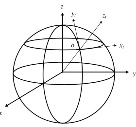
Tangential Cartesian Coordinates

The tangential Cartesian coordinates can be established on the surface of the earth, as shown in Figure 2.1. The origin of this coordinate system is located at a position O on the earth's surface. The x_t and y_t axes form a plane tangent to the earth's surface and

point towards the east and the north, respectively. The z_t axis points in the radial

(46)

Figure 2.1. Tangential Cartesian Coordinates

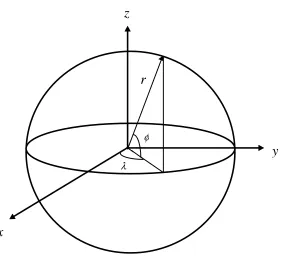
Spherical Coordinates

The geometry of the earth is nearly spherical with slight ellipticity. In common practice, the earth is taken to be a sphere with associated spherical coordinates. As discussed in Haltiner and Williams [27], use of these coordinates in global models of atmospheric transport of chemical species has gained acceptance. These coordinates

(

r,λ φ,

)

are shown in Figure 2.2.

y

x

z

t

o

y

t

(47)

Figure 2.2. Spherical Coordinates

Map Projections

It is useful to project the surface of the earth onto a plane for analysis and visualization. The most popular projections are Polar Stereographic at high latitudes, Lambert Conformal at mid-latitudes, and Universal Transverse Mercator (UTM) near the equator. When doing a projection, new horizontal coordinates are set up on the projected plane and the governing equations and associated initial and boundary conditions are transformed accordingly. A good description of map projections is provided in Haltiner and Williams [27].

r

y

x

z

(48)

2.3.2 Vertical Coordinate Systems

The vertical structure of the atmosphere suggests that it might be useful to replace the geometrical vertical coordinate by one of the flow variables and, thus, use a generalized vertical coordinate in meteorological modeling. This generalization of the vertical structure of the atmosphere can provide simplifications in modeling procedures and allow terrain following. Several vertical coordinates in use have been discussed in Kasahara [28]. Since a meteorological model provides the meteorological inputs (boundary layer characteristics, cloud structure, wind patterns, etc.) for an AQM, it is important that an AQM have a coordinate system that is compatible with the meteorological model. Otherwise errors in meteorological input data for AQM will result from transforming this data from the coordinate system of the meteorological model to that of the AQM. Some popular vertical coordinates are summarized in Table 2.1 given below.

2.3.3 Coordinate Transformations

(49)

Toon et al. [23], and McRae et al. [17]. In this work, a cohesive treatment of some of the coordinate systems used in AQMs is provided in Appendix A.

Table 2-1. Some Generalized Vertical Coordinates

Vertical Coordinate Reference Remarks

Altitude Toon (1988)

Pressure Toon (1988)

Sigma-p:

σ p =

p − p _T p _S− p _T

Chang (1990) pS( , )x y is surface

pressure, p _T is top layer pressure

Sigma:

σ = p −₋p

p p

T

S T

0

Grell (1993) p z0( ) is reference

pressure, ρ ₀( z ) is reference air density

Sigma-z:

σz

z h H h

= −

−

McRae (1982) h x y( , ) is lower surface,

H x y t( , , ) is height of upper surface

Scaled height:

(

)

z H z z

H z

s s

= ₋−

(50)

3

Elements of DSAGA-PPM

DSAGA-PPM includes the finite volume procedures for advancing the governing system (i.e., Equation (2.13) and the associated initial and boundary conditions) in time using a non-uniform grid, for moving the grid nodes to region(s) requiring solution refinement, and for conservatively redistributing the solution field over the resulting adapted grid. These procedures are described below.

3.1

Time Advancement of the Governing System

In the AQMs based on finite volume methods, the governing system, with transformed vertical coordinate, is usually advanced in time on static Cartesian grids with uniform spacing in the horizontal plane and non-uniform spacing in the vertical direction. However, in general, an adapted grid will not be uniform. Therefore in DSAGA-PPM, the solutions of the governing system need to be obtained on non-uniform grids. To facilitate this, a coordinate transformation is applied to the governing system to move from the physical domain expressed in Cartesian coordinates (x, y, z) to a computational

domain expressed in general curvilinear coordinates ( , , )ξ η ζ . The grid in these general

(51)

In physical space, Equation (2.13) can be expressed in Cartesian coordinates as ∂ ∂ ∂ ∂ ∂ ∂ ∂ ∂ c t E x F y G

z R S l N

l l l l

l l

+ + + = + , =1,..., ; (3.1)

where:

E c u K c

x K

c

y K

c

z l N

l l xx

l

xy l

xz l

= − ∂_∂ − ∂_∂ − ∂_∂ , =1,..., ; (3.2)

F c v K c

x K

c

y K

c

z l N

l l yx

l

yy l

yz l

= − ∂_∂ − ∂_∂ − ∂_∂ , =1,..., ; (3.3)

and

G c w K c

x K

c

y K

c

z l N

l l zx

l zy l zz l = − ∂ − − = ∂ ∂ ∂ ∂

∂ , 1,..., . (3.4)

With the assumption of diagonal K (see Section 2.1), the above expressions reduce to

E c u K c

x l N

l l xx

l

(52)

F c v K c

y l N

l l yy

l

= − ∂_∂ , =1,..., ; (3.6)

and

G c w K c

z l N

l l zz

l

= − ∂ =

∂ , 1,..., . (3.7)

The mapping between the physical space expressed in Cartesian coordinates and the computational space expressed in general curvilinear coordinates ( , , )ξ η ζ is given by

ξ ξ= ( , , ),x y z η η= ( , , ),x y z ζ ζ= ( , , )x y z . (3.8)

As discussed in Roache [29], in general, the most accurate numerical results are obtained if numerical differencing is based on the conservative form of the governing equations. Methods for manipulating partial differential equations that preserve conservative properties are described in Anderson et al. [30], Oberkampf [31], and Vinokur [32]. Using these methods, it is possible to arrive at the conservative form of the transformed atmospheric diffusion equation given by

∂ ∂

∂ ∂ ξ

∂ ∂ η

∂ ∂ ζ

$ $ $ $ _$ _$

, ,...,

c

t

E F G

R S l N

l l l l

l l

(53)

where:

$ / , ,...,

cl =cl J l=1 N ; (3.10)

$ ₍ _{) / ,} _,...,

E_l E F G J l N

x y z

= ξ +ξ +ξ =1 ; (3.11)

$ ₍ _{) / ,} _,...,

F_l E G G J l N

x y z

= η +η +η =1 ; (3.12)

$ ₍ _{) / ,} _,...,

G_l E F G J l N

x y z

= ζ +ζ +ζ =1 ; (3.13)

$ ( ,..., ) / , ,...,

R_l = R c_l ₁ c_N J l =1 N; (3.14)

and

$ ₍ _{, ) / ,} _,...,

Sl =S X tl J l= N

r

1 . (3.15)

The expressions for the Jacobian J and the metrics of the transformation are available in Anderson et al. [30] and are also provided in Appendix B.

(54)

decoupling transport and chemistry and solving for these processes in sequential steps results in more efficient computation of transport. As discussed in [17], Equation (3.1) (or Equation (3.9)) is operator - (or time -) split [33] to compute transport, chemistry, and source processes in sequential steps. The splitting of Equation (3.9) is not unique and differs between AQMs. One possible splitting sequence is

c tl( +∆t)= L L Lc_l s_l diff Lζ,advLη,advLξ,avdc tl( ), l =1,...,N ; (3.16)

c tl( +2∆t)= Lξ,advLη,advLζ,advLdiffL L c ts_l c_l l( +∆t), l=1,...,N; (3.17)

where:

L J u v w

J adv

x y z

ξ _{∂ ξ}∂

ξ ξ ξ

,

( ) ( ) ( )

=  − + − + −



 



 ; (3.18)

L J u v w

J adv

x y z

η _{∂ η}∂

η η η

,

( ) ( ) ( )

=  − + − + −



 



; (3.19)

L J u v w

J adv

x y z

ζ _{∂ ζ}∂

ζ ζ ζ

,

( ) ( ) ( )

=  − + − + −



 



(55)

L J K c x K c y K c z J diff x xx l y yy l z zz l = + +             + ∂ ∂ ξ ξ ( ∂_∂ ) ξ ( ∂_∂ ) ξ( ∂_∂ ) J K c x K c y K c z J x xx l y yy l z zz l ∂ ∂ η η ( ∂_∂ )+η ( ∂_∂ )+η( ∂_∂ )             + J K c x K c y K c z J x xx l y yy l z zz l ∂ ∂ ζ ζ ( ∂_∂ )+ζ ( ∂_∂ )+ζ ( ∂_∂ )             (3.21)

( )

L_s S X t_l l N

l = =

r

, , 1,..., ; (3.22)

and

(

)

Lc_l = R cl 1,...,cN , l =1,...,N. (3.23)

(56)

With this splitting, high resolution advection solvers, developed for one-dimensional Euler equations, can be used to compute time-split three-dimensional advection.

The remainder of this chapter develops application of DSAGA-PPM to the atmospheric diffusion equation in two-dimensions only. Application of this algorithm to the atmospheric diffusion equation in three-dimensions be a logical extension of the procedures presented in the following sections.

3.2

Treatment of Two - Dimensional Advection

The finite volume representation of the advection component of (3.9), with splitting (3.16) and (3.17), can be used to compute two-dimensional advection. Accordingly, the advection solution at t+ ∆tis given by

( ( ) )_, ( ) ( $ $ ) , ,...,

/ , / ,

,

c_l n V _{i j} c V_ln _{i j} t_adv E_ladv E l N

i j l

adv

i j

n +

+ −

− + − = =

1

1 2 1 2 0 1

∆ ; (3.24)

( )_, ( ( ) ) ( $ $ ) , ,...,

, / , /

( )

,

c_ln V _{i j} c_l n V _{i j} t_adv F_ladv F l N

i j l

adv i j

n

+ +

+ −

+

− + − = =

1 1

1 2 1 2

1

0 1

(57)

with

$

/ ,

/ , E

J uc J vc

l adv i j x l y l i j + + = +      1 2 1 2 ξ ξ ; (3.26) and $ , / , / F

J uc J vc

l adv i j x l y l i j + + = +      1 2 1 2 η η . (3.27)

In Equations (3.24) through (3.27), c_l is the average concentration of chemical species l

in cell volume Vi, j ; E$l adv

and F$_ladv are the net mass effluxes due to advection at cell sides

i±1 2/ , j and i, j±1 2 , respectively; and / (n+1) is an intermediate time level

between the levels n and n+1 . Note that the concentrations appearing in Equations (3.26) and (3.27) have to be evaluated at the appropriate cell sides. For example, c_l

appearing in Equation (3.26) has to be evaluated at the cell side i+1 2/ , j. In a finite

volume formulation, the Jacobian J is simply the ratio of the volume of the computational cell to the volume, V, of the corresponding physical cell. In the computational domain, the grid is chosen to be uniform and unit-spaced for convenience. Consequently, the volume of each computational cell is unity and the Jacobian for each

cell becomes 1

(58)

In air quality simulations, mass conservation of species, monotonicity of the solution fields, and high order of accuracy need to be maintained during numerical computations. The Piecewise Parabolic Method (PPM) - a numerical scheme for computing advection - is monotonic, is third order accurate for variable grid spacing, and has excellent mass conservation property [34]. Therefore, a time split version of the PPM

scheme is used to compute the fluxes E$_ladv and F$_ladv required in (3.24) and (3.25). The PPM scheme, developed for modeling fluid flows with strong shocks and discontinuities, is a higher-order extension of Godunov’s method and uses a parabola as the basic interpolation function in a finite volume cell [16]. A description of the PPM scheme is presented in Appendix C.

(59)

sources resulting from the difference algorithm. Subsequently, these sources are eliminated by adding terms equal to negative of numerical source terms to the difference equations. In DSAGA-PPM, this procedure was used to eliminate the advective numerical sources, as described below.

Equation (3.24) is rewritten to yield

c c t

V E E l N

l n

i j l

n i j

adv i j

l adv

i j l

adv

i j

n

( )

, ,

, / , / ,

( $ $ ) , ,...,

+

+ −

= − − =

1

1 2 1 2 1

∆

. (3.28)

In the above equations, $

/ ,

E_ladv

i+1 2 j and

$

/ ,

E_ladv

i−1 2j are the advective mass fluxes at

the cell edges i+1 2/ , j and i−1 2/ , j, respectively. As described before, in

DSAGA-PPM these fluxes are computed using the DSAGA-PPM scheme. For a flow with uniform (or constant) dependent variables cl, the PPM scheme reduces to the first order upwind

(60)

Expanding Equation (3.28) for the uniform dependent variable flow,

c c

t c

V J u J v J u J v l N

l n

i j l

n i j adv l n i j i j x y i j x y i j n ( ) , , , , _{/ ,} _{/ ,} , ,..., . + + − = − ⋅  +      − +              = 1

1 2 1 2

1

∆ _ξ _ξ _ξ _ξ

(3.29)

Upon inspection of the above equations for a constant dependent variable flow, the numerical source term is identified to be

− ⋅  +      − +              = + −

∆t c

V J u J v J u J v l N

adv l n i j i j x y i j x y i j n , , _{/ ,} _{/ ,} , ,..., ξ ξ ξ ξ

1 2 1 2

1 . (3.30)

Subsequently the negative of this term is added to (3.24) to eliminate numerical sources. A similar source correction is applied to (3.25).

The time step for advection is calculated as follows. Considering Equation (3.9), one dimensional advection is expressed as:

∂ ∂ ∂ ∂ ξ ξ ξ $ $ $ ; $ , $ c t u c c c

J u u v

l l

x y

(61)

As shown in Anderson et al. [30], for the explicit upwind method being used to solve the above equation, stability consideration requires that

(

$

)

/ ,

u t_adv

i j

∆ ∆

+1 2 _≤

1

ξ . (3.32)

Rearranging the above relation,

∆t ∆ ∆

u

adv i j

i j + + ≤ = 1 2 1 2 1 / , / , $ ; ξ _ξ . (3.33) Then, ∆t

J u J v J

adv i j

x y i j + + ≤ +               1 2 1 2 1 / , / ,

ξ ξ . (3.34)

The metrics ξx

i j

J ₊_{1 2}_{/ ,} and

ξy

i j

J ₊

1 2/ ,

are obtained using the relations given in Appendix B.

(62)

(

)

J

x y y x

J J J J

i j

i j x

y y _x

i j + + + = − =  ₋      1 2 1 2 1 2 1 1 / , / , / , ξ η ξ η ξ η ξ η ; (3.35) where

η _x η η η η

i j x i j x i j x i j x i j

J J J J J

+ + − + + + − = ⋅ + + +       

1 2 1 2 1 2 1 1 2 1 1 2

0 25

/ , , / , / , / , /

. ; (3.36)

and

η _y η η η η

i j y i j y i j y i j y i j

J J J J J

+ + − + + + − = ⋅ + + +       

1 2 1 2 1 2 1 1 2 1 1 2

0 25

/ , , / , / , / , /

. . (3.37)

Then using Equation (3.34), the time step for each of the cell edges i±1 2/ , j is

obtained. In a similar fashion, the time step for each of the cell edges i j, ±1 2 is/

obtained. Finally,

∆t_adv ∆t_{adv i} ∆t i j

j adv i j

= min( ₊ , ₊ ) ∀ ,

/ , , /

1 2 1 2 . (3.38)

(63)

3.3

Treatment of Two - Dimensional Turbulent Diffusion

The finite volume representation of the turbulent diffusion component of (3.9), with splitting (3.16) and (3.17), can be used to compute two-dimensional turbulent diffusion. Accordingly, the turbulent diffusion solution at t+ ∆tis given by

( ) ( )

( $ $ $ $ ) , ,..., ;

,

/ , / , , / , /

,

c V c V

t E E F F l N

l n

i j l

n i j

diff l diff

i j l