An Empirical Process for Building and Validating Software
Engineering Parametric Models
Mark Sherriff
1, Barry Boehm
2,
Laurie Williams
3, and Nachiappan Nagappan
4Abstract
Parametric modeling is a statistical technique whereby a dependent variable is estimated based on the values of and the relationships between the independent variable(s). The nature of the dependent variable can vary greatly based on one’s domain of interest. In software engineering, parametric models are often used to help predict a system’s development schedule, cost-to-build, and quality at various stages of the software lifecycle. In this paper, we discuss the use of parametric modeling in software engineering and present a nine-step parametric modeling process for creating, validating, and refining software engineering parametric models. We illustrate this process with three software engineering parametric models. Each of these models followed the nine-steps in different ways due to the research technique, the nature of the model, and the variability of the data. The three models have been shown to be effective estimators of their respective independent variables. This paper aims to assist other software engineers in creating parametric models by establishing important steps in the modeling process and by demonstrating three variations on following the nine-step process.
1 INTRODUCTION
Parametric modeling is a statistical technique whereby a dependent variable is estimated based on the relationships between and the values of the independent variable(s) (Gallagher 1982). The nature of the dependent variable can vary greatly based on one’s domain of interest. The importance of predicting how phenomena will behave in the future ranges from convenience to life-critical. Every time a person makes a decision on what he or she will do the next day based on the weather report, including serious predictions such as an impending hurricane, is relying on a type of parametric model (Coles and Tawn 1991). Businesspeople make decisions about the stock market or how a project should proceed based on profit predictions that they receive. In engineering and the sciences, research has been performed to establish parametric models to estimate everything from energy consumption (Hall 1997) to railway line capacity (Prokopy 1975) to the physics of approaching aircraft (Moen 1976). Government agencies, such as the Department of Defense, along with the International Society of Parametric Analysts, use parametric analysis when creating proposals and has seen that it helps to improve cost predictions (International Society of Parametric Analysts 2003).
In software engineering, parametric modeling has been used for prediction (Sherriff, Boehm et al. 2005), e.g. the costs of and resources for building software, such as the number of person-hours to complete a project
(Boehm, Horowitz et al. 2000) and the potential reliability of a system in an early stage (Nagappan 2005; Sherriff, Nagappan et al. 2005). In this paper, we will discuss the use of parametric modeling in software engineering and present a nine-step parametric modeling process for creating, validating, and refining software engineering parametric models. The underlying concepts laid out in the process are intended as a basic guideline for those desiring to create their own parametric model in a software engineering domain. These steps can and should be done iteratively, proceeding through the process once, and then revisiting steps and revising later once more information is available. When the steps are revisited with more information, the model will improve.
We illustrate the modeling process with three software engineering parametric models that have been created and validated using this nine-step process. These three models are the Constructive Cost Model (COCOMO) II (Boehm, Horowitz et al. 2000) to estimate project costs; the Software Testing Reliability Early Warning model for Java (STREW-J) (Nagappan 2005) to estimate trouble reports (TR) (Mohagheghi 2004) per thousands of lines of code (KLOC); and the Software Testing Reliability Early Warning model for Haskell (STREW-H) (Sherriff, Nagappan et al. 2005) to estimate post-release defect density. These three models help to show that, while the complexities of these three software engineering parametric models are vastly different, the underlying concepts behind these models are fundamentally domain independent. Each of these models followed the nine-steps in different ways due to the research technique, the nature of the model, and the variability of the data. The three models have been shown to be effective parametric models.
The remainder of this paper is organized as follows. Section 2 describes an overview of the current state of parametric modeling in software engineering. Section 3 presents a nine-step parametric modeling process for software engineering. Sections 4, 5, and 6 illustrate example parametric models that utilized the process described in this paper, while Section 7 summarizes these sections. Section 8 presents conclusions and future work.
2 OVERVIEW OF PARAMETRIC MODELING
The overall purpose of parametric models is to make an estimation or prediction based on current information. In the general sense, a function y = f(x1, x2, x3, …) is created such that xi is an input to the function and y is the variable being estimated. Some examples of the types of relationships in parametric modeling are (Boehm 2003):
• Analogy: Outcome = f(previous outcome, difference) – used to make a prediction based on what happened before and then taking into account the differences in the scenario. Examples: weather prediction; traffic patterns
• Unit Cost: Outcome = f(unit costs, unit quantities) – used to make a prediction based on known production values. Examples: potential profit based on units available to be sold.
• Relationship-Based: Outcome = f(parametric relationships) – used to make a prediction based on the relations and interactions of inter-dependant variables. Examples: predicting heart disease based on height, weight, and family history; software size/cost models
Parametric models may be calibrated for use in a particular situation, organization, or even particular project (Gallagher 1982). For example, while person-hours might be a heavy contributor to cost for one particular project, another project might rely more heavily on state-of-the-art technology, and thus technology expenditures might play a larger role in cost. Some parametric models are robust enough or have been built with a large amount of data to be sufficient for use in many projects, such as COCOMO II (Boehm, Horowitz et al. 2000). However, some models may remain domain- or context-dependant, such as STREW-J (Nagappan 2005)and STREW-H (Sherriff, Nagappan et al. 2005), due to smaller amounts of data or to large differences in domains.
3 PARAMETRIC MODELING PROCESS
Figure 1. Parametric Modeling Process for Software Engineering
Step one: Determine model needs. The general goal for creating a parametric model in software engineering is to help provide an estimation or prediction of an important product attribute early in the process so that development efforts can be directed accordingly. Some specific goals might be:
• To provide an estimate of post-release quality during the unit test phase without causing burden on the software engineers.
• To provide an estimate of how many programmers are needed to complete the product by a given date. Similar to gathering requirements in requirements engineering, the goal of the model must be defined at the beginning of the model creation process. First, the stakeholders in the success of the model need to be identified. Stakeholders include such people as project managers, the users of the model, the data providers for the model, and the model developers. Then, the model needs and specific success criteria must be identified. These criteria will provide the basis for showing that the model was created correctly and addresses the needs of the stakeholders.
provide an estimation of software cost, the model developers should have a deep understanding of each of the factors that can contribute to cost, such as person-hours, defect removal, and project management, and the metrics used to quantify these factors. Appropriate and, preferably, verified metrics that have been shown to be indicators of the dependent variable become candidate metrics. One way to approach the analysis of existing literature is through a systematic review (Kitchenham 2004). A systematic review is a methodology by which research and references on a particular topic are evaluated and interpreted for use in other work. The difference between a systematic review and a simple literature review is that a systematic review is a specific kind of literature review in which a predefined search strategy is followed and each resource is evaluated by set criteria to determine its value (Kitchenham 2004). This process helps ensure that all proper references and information are examined in a methodical way and are considered appropriately.
Step three: Perform behavioral analysis. Model developers can add to and refine the list of candidate metrics by doing a behavioral analysis of the variable to be estimated. With an understanding of the background and phenomenology of the dependant variable, developers can theorize as to what different behaviors of various factors could have on the dependent variable. This analysis of these behaviors is another way for model developers to triangulate on a set of candidate metrics. For example, Table 1 demonstrates a behavioral analysis of software reliability based upon the practices of requirements specification and testing. Using the extremes of “very low” and “very high” reliability, a comparison of the typical characteristics of requirements specifications and testing practices that would yield a high or low reliability product is made. Through this comparison, the model developer can ensure the essential differences between good and bad “behavior” of the value to be estimated are captured in the candidate metrics.
Table 1. Behavior differences for required reliability levels.
Rating Very Low Reliability Very High Reliability
Requirements
Specification •• Little detail Many open items
• Little verification
• Minimal quality assurance (QA)
• Detailed verification standards
• Detailed test plans and procedures
Testing • No test procedures
• Many requirements untested
• Minimal QA
• Minimal stress / off-nominal tests
• Detailed test procedures and QA
• Extensive stress / off-nominal tests
Step four: Define relative significance. Metrics are given a relative ranking, such as High, Medium, and Low, as to what effect they are expected to have on the model as a whole. Based on previous research or anecdotal evidence, model developers should be able to theorize about what effect different levels of each metric will have on the estimate the model provides. For example, model developers might consider how requirements volatility would affect defect density.
Step five: Gather expert opinion. Domain experts can help refine the candidate metrics to add their experience to the model. Qualifications for experts will vary between domains. For example, the experts used in the studies presented in this paper had at least five years experience in their particular field, and were solicited from the domain community. Specifications for who would qualify as an expert should be addressed at the beginning of this step. Experts are likely to uncover factors that were not included, over- or under- emphasized, overlap with others, or are incorrect for this use.
Step six: Formulate a priori model. A rubric for evaluating and recording parameter values from actual projects can be created such that the initial version of the model may be proposed. This initial version of the model is not calibrated and cannot yet be used to generate an accurate prediction. The most important part of this initial model is a detailed description of the techniques that will be used to gather each metric. This detailed description should outline exactly what each metric is, what tools are used to gather each metric, and specific instructions as to how to perform the data gathering.
Step seven: Gather project data. Metrics can now be gathered on the software project. This data should be gathered from similar projects within an organization. These projects would ideally be in the same domain, with the same constraints, and a similar development team. If optimal projects are not available, similar projects from other organizations, or internal projects of a somewhat similar domain with the same development team could be used. The previous projects used in data gathering should be as similar as possible to the project(s) that the model will be used to estimate. Data gathering should be a collaborative effort between the model developers and the data providers. This collaboration will help clarify any ambiguities that were not eliminated during earlier steps in the process, and the data collection rubric can be refined (re-visiting step six). Depending on the complexity of the metrics, the number of projects, the development cycle of the project, and the ease of collecting the metrics, data gathering can take from one week to several months.
Step eight: Calibrate a-posteriori model. After the initial metric data and actual values for the dependent variable have been gathered, the parametric model can be calibrated to the organization utilizing the model. Various techniques have been used for model calibration, including Bayesian analysis (Gelman, Garlin et al. 1995), regression analysis (Munson 1990), and exhaustive search through the set of all possible calibration values (Menzies, Port et al. 2005). Bayesian analysis is a statistical technique that uses expert judgment along with sampling information to make an efficient model (Devnani-Chulani 1999). Regression analysis yields a multiple coefficient of determination, R2, which provides a quantification of how much variability in the data can be explained by the regression model. One difficulty associated with regression analysis is multicollinearity among the metrics.
four projects and then used this model to predict person-hours in 56 other projects. For general parametric models, calibration could continue until there is no significant improvement in the accuracy of the model. The number of data points necessary could vary from model to model, depending on the number of parameters and the overall variability of the data.
Step nine: Gather more data and refine model. More data from other sources needs to be introduced to further refine the model. For instance, data from projects that have had values estimated should be added to the model when actual values for the estimated variables are available. These new data can prompt the return to any of the above steps to discover how the model might be changed so that it might be improved. Model accuracy can be improved by adding new data. Also, metrics might be identified at this stage that do not significantly add to the model and can thus be removed to minimize the number of metrics and decrease the overhead of metrics collection. Also, if projects are added to the model that are somewhat different, the model could be more robust in the types of projects that can be estimated.
In the next three sections, we illustrate these nine steps by explaining how each of the steps was applied in the development and refinement of three parametric models for software engineering.
4 COCOMO II
This section discusses the creation of COCOMO by Barry Boehm. COCOMO (Boehm 1981) is a model for estimating cost, effort, and schedule when planning a new software development activity. The COCOMO research has spawned other similar models, such as Constructive Commercial-of-the-shelf (COCOTS) Model (Abts, Boehm et al. 2000), Constructive Quality Model (COQUALMO) (Devnani-Chulani 1999), and Constructive System Engineering Model (COSYSMO) (Valerdi, Miller et al. 2004) which provide specialized information regarding commercial software development, software quality, and large-scale software and hardware projects, respectively. In this section, we will show how the second iteration of COCOMO, COCOMO II, was created and how it evolved into its current form (Boehm, Horowitz et al. 2000). COCOMO II consists of three sub-models, each one offering a more detailed view of a project based on how far along the development team is during design and coding (Boehm, Horowitz et al. 2000). We will focus on the Post Architecture sub-model of COCOMO II, which is used when top-level design is complete and detailed information about the project is available.
4.1 Step one: Determine model needs
data points collected in 1979. COCOMO 81 was adapted and used by numerous major organizations around the world for estimating cost components of software development.
However, as new software development techniques arose, it became clear that many of the assumptions underlying the original COCOMO 81 model were not well matched to the new ways that software was being developed. New technologies and techniques such as specialized development methodologies and module reuse were not handled adequately in the COCOMO 81 parameters. The organizations around the world that had been using COCOMO 81 needed to have an updated version of the model to continue to make project cost decisions in the future. These essential model stakeholders, including the model developers and representatives from organizations that were affiliates of the Center for Software Engineering5 at the University of Southern California, began the COCOMO II (Boehm, Horowitz et al. 2000) project in 1997 to update COCOMO 81 for the future. The model developers aimed to provide a new version of COCOMO that was better tuned to current and likely future software practices, while preserving the open nature of COCOMO's internal algorithms and external interfaces.
The main goals for COCOMO II were to provide cost and schedule estimates for current and future software projects and to be flexible enough to be tailored to a specific organization (Boehm, Horowitz et al. 2000). Success would be determined by the accuracy of these predictions.
4.2 Step two: Analyze existing literature
The first step in modifying the first iteration of COCOMO, COCOMO 81, to COCOMO II was to perform a comparative analysis of the software development approaches taken by the leading commercial software cost models. The model developers also performed a forecast of future software development processes, which indicated that cost models would need to address projects using a mix of process models. Other concepts and technologies that would need to be addressed included sophisticated forms of reuse, COTS integration, GUI builders, object-oriented methods, and Internet-based distributed development.
For COCOMO II, twenty-two parameters were determined based on data from the usage of the COCOMO 81 model and research that had been performed on it in previous years (Boehm, Horowitz et al. 2000). First, the COCOMO 81 parameters were analyzed to determine if they would be retained in the COCOMO II model. Eleven parameters were directly translated to the new model. Other parameters were then combined or modified to adjust for the newer development techniques that COCOMO II would address beyond COCOMO 81. Finally, new parameters were added to complete the assessment of the newer development techniques.
4.3 Step three: Perform behavioral analysis
A behavioral analysis was then performed to determine if there were other cost factors that had not been addressed. Overall categories were derived to classify the different cost factors. For COCOMO II, the effects of each of the 22 COCOMO II factors on productivity were analyzed qualitatively and classified (Devnani-Chulani 1999). The detailed results of this analysis can be found in (Devnani-(Devnani-Chulani 1999). The results of
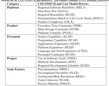
this study indicated that the model developers had sufficiently addressed the different factors in predicting project cost. The initial set of predictor parameters was then derived and is shown in Table 2.
Table 2. Initial set of COCOMO II parameters. (Devnani-Chulani 1999; Boehm, Horowitz et al. 2000)
Category COCOMO II and Cost Model Drivers
Platform Required Software Reliability (RELY) Data Base Size (DATA)
Required Reusability (RUSE)
Documentation Match to Life-Cycle Needs (DOCU) Product Complexity (CPLX)
Product Execution Time Constraint (TIME)
Main Storage Constraint (STOR) Platform Volatility (PVOL)
Personnel Analyst Capability (ACAP)
Programmer Capability (PCAP) Applications Experience (AEXP) Platform Experience (PEXP)
Language and Tool Experience (LTEX) Personnel Continuity (PCON)
Project Use of Software Tools (TOOL)
Multisite Development (SITE)
Required Development Schedule (SCED) Scale Factors Precedentedness (PREC)
Development Flexibility (FLEX) Architecture/Risk Resolution (RESL) Team Cohesion (TEAM)
Process Maturity (PMAT)
4.4 Step four: Define relative significance
The relative significance of each cost driver on productivity was determined for COCOMO II (Devnani-Chulani 1999). The COCOMO II parameters and the factors that form the parameters were rated from low to high as to their effect on the development effort. For example, requirements understanding (indicated as RELY) was rated as high, while process maturity (indicated as PMAT) was rated from low to medium. These efforts gave the model developers an early indication of how the model parameters of which parameters might be emphasized in the model and how they might interact together to provide a cost estimate for software engineers.
4.5 Steps five and six: Gather expert opinion & formulate a-priori model
The data from this first round was collected and refined. The experts were then presented with an opportunity to revise their numbers based on the submissions of the other experts during the second round of the Delphi process. The detailed results of this study (Devnani-Chulani 1999) show that the initial set of parameters described in Table 2 were acceptable and were representative of real-world phenomena in the development of software systems (Chulani, Boehm et al. 1999).
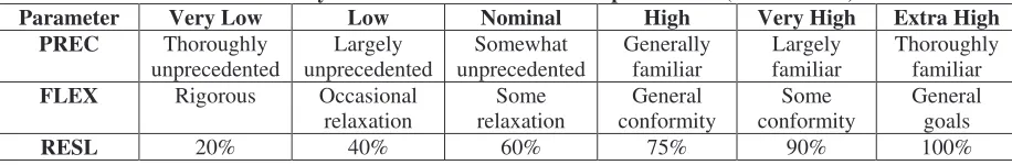
A rubric was defined for each of the COCOMO II parameters for the surveys that would be used to gather the data. Model developers and industry experts took each parameter in Table 2 and defined six levels that could be measured for each. The goal was to create a survey that could be easily understood by the different project managers and cost experts that would be taking the survey to provide the data for COCOMO II. An example set of parameters can be seen in Table 3.
Table 3. Survey rubric of three COCOMO II parameters (Boehm 2003).
Parameter Very Low Low Nominal High Very High Extra High
PREC Thoroughly
unprecedented unprecedented Largely unprecedented Somewhat Generally familiar familiar Largely Thoroughly familiar
FLEX Rigorous Occasional
relaxation relaxation Some conformity General conformity Some General goals
RESL 20% 40% 60% 75% 90% 100%
4.6 Step seven: Gather project data
From 1994 to 1997, data was gathered from 83 projects from commercial, aerospace, government, and non-profit organizations (Devnani-Chulani 1999). These organizations were affiliates of the Center for Software Engineering at the University of Southern California. A survey form (Devnani-Chulani 1999) was used to gather and record the data. This survey contained between 33 and 59 questions that varied by how much code reuse an organization had (Clark, Devnani-Chulani et al. 1998). All the data that was collected was from completed projects. Data collectors gathered this information through phone interviews, site visits, or through submission of completed forms. Overall, the 83 data points ranged from 2 to 1300 KLOC in size, 6 to 11,400 person months, and were completed over 4 to 180 months (Clark, Devnani-Chulani et al. 1998). While this initial iteration of COCOMO II included these 83 projects, the total dataset currently for COCOMO II calibration exceeds 200 projects (Boehm, Horowitz et al. 2000).
4.7 Step eight: Calibrate a-posteriori model
Using the data from the 1997 surveys of 83 completed projects, COCOMO II was calibrated using a multiple regression analysis (Clark, Devnani-Chulani et al. 1998; Devnani-Chulani 1999). The value being estimated was human resources, in terms of person months, as a linear function of the various parameters mentioned in Section 4.2. Equation 1 shows the regression equation created for COCOMO II:
∏
×
×
=
= = − 17
1 3
1 01 . 1
]
[
i i
SFi
EMi
Size
A
where, A = Baseline multiplicative calibration constant; B = Baseline Exponential calibration constant, set at 1.01 for the 1997 calibration; Size = Size of the software project measured in terms of KLOC or Function Points; SF = Scale Factor; and EM = Effort Multiplier (Devnani-Chulani 1999; Boehm, Horowitz et al. 2000). This particular iteration of the COCOMO II model was shown to be able to provide estimates within 30% of the actual human resource usage 60% of the time (Chulani, Boehm et al. 1999).
The results of this study showed that some parameters were highly correlated, and it was decided to combine them to reduce the effort need to use the model. These parameters included Analyst Capability and Programmer Capability (correlation coefficient of .7339), which were aggregated into Personnel Capability (PERS); and Time Constraints and Storage Constraints (correlation coefficient of .686), which were aggregated into Resource Constraints (RCON) (Devnani-Chulani 1999). The next highest correlation (0.62) was between Precedentedness (PREC) and Development Flexibility (FLEX). These two variables were not combined because the threshold value for combining parameters was a correlation coefficient of at least 0.65 (Clark, Devnani-Chulani et al. 1998; Boehm, Horowitz et al. 2000).
4.8 Step nine: Gather more data and refine model
Based on the cost model review and technology forecast, a series of iterations began with the organizations involved with the development of COCOMO II to continue to gather data to converge on a set of functional forms and baseline cost drivers for the model. The parameters themselves were deemed acceptable, but the model could be improved through a larger data set and with a better calibration technique. To improve the calibration process, Devnani-Chulani investigated calibrating COCOMO II using Bayesian analysis (Devnani-Chulani 1999). During Bayesian analysis, initial data is used to create a post-data model that “learns” as more data is added back into it, using Bayes’ theorem. This calibration technique provided a different set of coefficients for the parameters in the model. More data was gathered from industry and government partners to create a new data set of 161 data points in 2000 (Devnani-Chulani 1999).
4.9 Step eight: Calibrate a-posteriori model – iteration 2
Using the data collected from the latest set of surveys taken in 2000, the next iteration of COCOMO II (COCOMO II.2000 (Boehm, Horowitz et al. 2000)) was calibrated using a Bayesian analysis, as opposed to the regression analysis used in the previous iteration (Chulani, Boehm et al. 1999).
For regression analysis to calibrate models with over twenty parameters, such as COCOMO II, with somewhat noisy software project data, it is likely that some of the determined parameters have weak statistical significance. In such cases, if one also has the means and variances of the parameter values resulting from an expert-group Delphic process, a Bayesian combination of the data regression results and the expert Delphic results can produce a more robust result. With the Bayesian combination, the a-posteriori parameter value will be closer to the more strongly-determined of the data-determined and expert-determined parameter values.
data, the resulting model produces estimates within 30% of the actual value 80% of the time. The models produced with COCOMO II.2000 are a significant improvement over the first iteration of COCOMO II, which could provide estimates within 30% of the actual values 60% of the time (Chulani, Boehm et al. 1999).
5 STREW-J
In this section, we illustrate the nine-step parametric modeling process by explaining the creation of the Software Testing Reliability Early Warning metric suite for Java (STREW-J). At the time of its initial creation, the developers of this model were not aware of early versions of the parametric modeling process. In a retrospective analysis, we find that the developers of this model created an effective model for estimating trouble reports in software and did, in fact, follow most of the steps of the parametric modeling process. As will be shown, several of the steps were revisited before a stable model was verified.
5.1 Step one: Determine model needs
In early 2003, Nagappan et al. began work on utilizing various software testing metrics to provide an estimate of software defect density. In industry, software defect density information becomes available too late in the development process to affordably guide corrective action. Further, actual defect density cannot be measured until a product has been completed and then provided to the customer for use. The longer a defect remains in a system, from design to coding to maintenance, the more expensive it becomes to correct the problem (Boehm 1981). Therefore, it would be highly beneficial for developers to receive information about software defect density earlier in the process.
The main stakeholders for STREW-J include the model developers and the developers and managers from the project teams that were involved in this study. The main goal of STREW-J is to provide an early estimate of software quality so that corrective action can be taken earlier in the development process to help improve overall software quality. The success criteria for the STREW-J model was that it should be able to predict defect density within 5% of actuals. The metrics of STREW-J focus on aspects of the system such as testing, complexity, and size. Prior studies (Vouk 1993; Basili, Briand et al. 1996; Chidamber 1998; Briand 1999; Tang 1999; Briand 2000; El Emam 2001; Subramanyam 2003) have all leveraged the structural aspects of the code to make an estimate of field quality. STREW-J utilizes structural aspects of the unit-testing effort as well.
5.2 Step two: Analyze existing literature
The initial research for the STREW metric suite was performed in the Java programming language. This was done due to the prevalence of Java and the use of automated testing tools, such as JUnit6, in academia and industry.
The initial STREW-J, Version 1.1 (Nagappan 2003), was formed using metrics derived from previous research found in literature. These metrics included:
•number of test cases/source lines of code (R1) is an indication of whether there are too few test cases written to test the body of source code;
•number of test cases/number of requirements (R2) is an indication of the thoroughness of testing relative to the requirements;
•test lines of code/source lines of code (R3) is an indication of whether the ratio R1 was misleading as there might have been fewer, but more comprehensive, test cases;
•number of assertions/source lines of code (R4) serves as a crosscheck for both R1 and R2 because there are few test cases but each have a large number of assertions. Assertions (Rosenblum 1995) are used in this metric as a means for demonstrating that the program is behaving as expected and as an indication of how thoroughly the source classes have been tested on a per class level;
•number of test classes/number of source classes (R5) is an indication of how thoroughly the source classes have been tested;
•number of conditionals (for, while, if, do-while, switch)/ number of source lines of code (R6) is an indication of the extent to which conditionals are used. The use of conditional statements increases the amount of testing required because there are more logic and data flow paths to be verified (Khoshgoftaar 1990);
•number of lines of code/number of classes (R7) is used as an indicator for estimating defect density when prior releases of the software are available so that any change in the relative class size can be analyzed to determine if the increase in the size of the class has be accompanied by a corresponding increase in the testing effort (El Emam 2001).
These metrics are intended to capture and evaluate the quality of the testing effort of a development team. R1-R7 all deal with the ratio of testing effort to some measure of project size, which could be indicative of whether testing efforts were substantial enough to remove most defects (Nagappan 2003; Nagappan 2005).
A review of pertinent literature indicated how different testing styles could potentially affect the STREW method. For example, the test quantification metrics are specifically intended to crosscheck each other to account for coding/testing styles. In this instance, one developer might write fewer test cases, each with multiple asserts (Rosenblum 1995) checking various conditions. Another developer might test the same conditions by writing many more test cases, each with only one assert. The metric suite is intended to provide useful guidance to each of these developers without prescribing the style of writing the test cases (Nagappan 2005). The use of the STREW-J metrics is predicated on the existence of an extensive suite of automated unit test cases being created as development proceeds. STREW-J leverages the utility of automated test suites by providing a defect density estimate.
5.3 Step three: Perform behavioral analysis
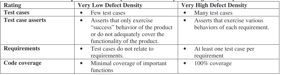
software defect density. Therefore, the behavioral analysis for STREW-J was focused specifically on how the different aspects of testing affected defect density. A sample of the behavioral analysis for defect density in a Java system as it relates to testing is shown in Table 4.
Table 4. Sample behavioral analysis for defect density for testing in a Java system.
Rating Very Low Defect Density Very High Defect Density
Test cases • Few test cases • Many test cases
Test case asserts • Asserts that only exercise “success” behavior of the product or do not adequately cover the functionality of the product.
• Asserts that exercise various behaviors of each requirement.
Requirements • Test cases do not relate to
requirements. • At least one test case per requirement
Code coverage • Minimal coverage of important
functions • 100% coverage
5.4 Step four: Define relative significance
For the development of STREW-J, relative significance was assigned to the parameters due to the desire to first gather initial data to explore the feasibility of building such a parametric model leveraging the testing effort. This initial project data would help to determine which parameters are more important in the model (Nagappan 2005). Based on our initial case study and follow up with industrial partners (Nagappan 2003) we determined that it was not possible to physically quantify requirements for commercial project. For this reason, the STREW-J metric involving requirements (R2) were removed from the initial model.
5.5 Step five: Gather expert opinion
During the initial creation of the STREW-J model, specific expert opinion was not gathered a priori. Expert opinion on the model was obtained from the community post-hoc during the peer-reviewed publication of “fast abstracts” of early versions of the work (Nagappan 2003; Nagappan 2003) in disseminating the results of the study.
5.6 Step six: Formulate a-priori model
The a-priori model for STREW-J was determined by applying the mathematical form of a regression analysis7, which would be carried out once data from the project had been collected. This is shown in Equation 2.
Defect density estimate= a + b*R1 + c*R2 + d*R3 + e*R4 + f*R5 + g*R6 + h*R7 (2)
Tools were also defined for gathering metrics. Borland’s Together IDE8 was used to gather some of the metrics, while other regular expression and line-of-code counting tools were used for the remainder.
7 SPSS was used for the purpose of statistical analysis. SPSS does not provide statistical significance beyond three decimal
5.7 Step seven: Gather project data
Once the initial model was created, the first feasibility study was performed to calibrate the model. The feasibility study was carried out in a junior/senior-level software engineering course at NCSU in the fall 2003 semester. Students developed an open source Eclipse9 plug-in in Java. Each project was developed by a group of four or five junior or senior undergraduates during a six-week final class project. The plug-in was required to have 80% unit test coverage via the JUnit unit test suite and for acceptance test cases to be automated via the FIT10 tool. A total of 22 projects were submitted; all were used in the analysis.
The plug-ins were evaluated using a comprehensive set of 31 black-box test cases. Twenty six of these were acceptance tests and were given to the students during development. The 31 test cases included exception checking, error handling, and five boundary test cases that checked the operational correctness of the plug-in. The Nelson model (Nelson 1978) was used as a baseline comparison with the defect density estimation to show the accuracy of the STREW-J model versus an established model.
5.8 Step eight: Calibrate a-posteriori model
Using the technique of data splitting, a random sample of 15 programs was selected to build the regression model, and the remaining seven programs were used to verify the prediction accuracy. The regression equation built had an R2 value of 0.405, (F=1.262, p=0.340) and is shown below in Equation 3.
Reliability Estimate = 1.114 - 0.0842*R1 - 0.0118*R2 - 0.0247*R3 + 1.954*R4 - 0.0036*R5 – 2.301*R6 - 0.0022*R7 (3)
5.9 Step nine: Gather more data and refine model
After the results of the initial STREW-J parametric model were reviewed and published, revisions were made to the metrics in the model. As will be discussed in Sections 5.10 and 5.11, a second literature search was conducted and more data was collected. Additionally, research began to focus on industrial and open source projects. The model developer altered the dependent variable for software quality from test failures/KLOC to trouble reports (TR) per KLOC to switch from a pre-release view of quality to a post-release (customer) view of quality. A TR (Mohagheghi 2004) is a customer-reported problem whereby the software system does not behave as the customer expects. A TR is a more accurate reflection of the post-release field quality of the system normalized by the size of the code base and independent of the operational profile of the software.
8 http://www.borland.com/together/
5.10 Step two: Analyze existing literature – iteration 2
The model developer analyzed the results of the feasibility study and returned to literature to refine and add new metrics to the STREW-J model. The metrics included in STREW-J Version 2.0 are shown in Table 5.
Table 5: STREW-J metrics Test quantification
Number of Assertions
SLOC* SM1
Number of Test Cases
SLOC* SM2
Number of Assertions
Number of Test Cases SM3
_____(TLOC+/SLOC*)___
(Number of ClassesTest Number of ClassesSource)
SM4
Complexity and O-O metrics
ΣCyclomatic ComplexityTest ΣCyclomatic ComplexitySource
SM5
ΣCBOTest
ΣCBOSource
SM6
ΣDITTest
ΣDITSource
SM7
Σ WMCTest
Σ WMCSource
SM8
Size adjustment
SLOC* ____________
Minimum SLOC* SM9
* Source Lines of Code (SLOC) is computed as non-blank, non-comment source lines of code
+ Test Lines of Code (TLOC) is computed as non-blank, non-comment test lines of code
release. The STREW-J metric suite is also used to provide color coded feedback (Nagappan 2005) to developers to identify areas that require further testing.
Further, drawing general conclusions from empirical studies in software engineering is difficult because any process depends to a large degree on a potentially large number of relevant context variables. For this reason, we cannot assume a priori that the results of a study generalize beyond the specific environment in which it was conducted (Basili, Shull et al. 1999). Researchers become more confident in a theory when similar findings emerge in different contexts (Basili, Shull et al. 1999).
5.11 Step seven: Gather project data – iteration 2
Data was gathered from 27 open source Java projects found on SourceForge11, an open-source development website, and five industrial projects from a company in the United States to calibrate STREW Version 2.0 (Nagappan 2005). The open source projects were selected from SourceForge based on their domain (all were software development tools), rate of active development, possession of automated unit tests, and TR logs availability. The size range of the open source projects was from one to almost 80 KLOC. These open source projects also had from one to hundreds of developers working on them at varying rates of development and with varying expertise.
The industrial case study involved three software systems (five versions) with a company in the United States. To protect proprietary information, the names and natures of the projects are kept anonymous. These projects were critical in nature because TRs could lead to loss of essential funds for the company. In the industrial environment, failures found by customers are reported back to the organization. These TRs are then mapped back to the appropriate software systems. Project sizes ranged from 13-504 KLOC, and team size varied from six to sixteen developers. Over half had at least five years experience working in this field.
Borland’s Together IDE was used to gather some of the complexity metrics, while other regular expression and line-of-code counting tools were used for the remainder. These metrics were then compiled for analysis.
5.12 Step eight: Calibrate a-posteriori model – iteration 2
The model developer used two-thirds of the open-source projects to build and calibrate the prediction model using a regression analysis and the remaining one-third to evaluate the fit of the model. Of the 27 projects, 18 projects were used to build the model and the remaining nine projects to evaluate the built model. The random split was conducted nine times to verify data consistency, i.e. to check if the results of the analysis were not a one time occurrence. This random-splitting was not performed with the academic projects feasibility study.
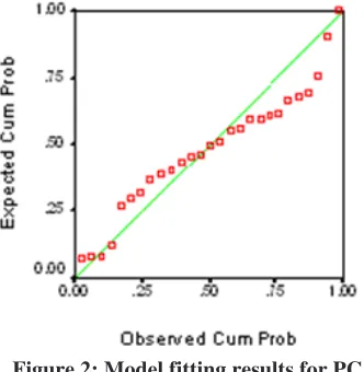
Principle component analysis (PCA) was used to help remove the multicollinearity exhibited in the STREW metrics model. For PCA to be applicable, the Kaiser-Meyer-Olkin (KMO) measure of sampling adequacy should be greater than 0.6 (Brace 2003). The KMO measure of sampling adequacy is a test of the amount of variance within the data that can be explained by the measures. The KMO measure of sampling adequacy was found to be 0.764 indicating the efficacy of the applicability of PCA. PCA of the nine STREW metrics yielded
two principal components. Thus, while the final STREW model uses the metrics listed in Table 5, they are converted into independent parameters (principle components) in the equation itself.
Figure 2 shows the complete model fit for all the 27 open source projects built using the principal components of the STREW metrics as the independent variable and the post-release failure density as the dependent variable. Similar to the academic case studies, the model built is statistically significant (R2=0.428, (F=8.993, p=0.004))
Figure 2: Model fitting results for PCA
The STREW model used was calibrated to the open source projects to predict the TRs of the industrial software systems. Figure 3 indicates the prediction plots obtained using PCA. The axes are removed to protect proprietary information.
Figure 3: Prediction plots with PCA
it. Even though the sample size is small (only 5 projects), the correlation results of the actual and estimated post-release failure density (Pearson correlation coefficient = 0.962 / p = 0.009 and Spearman correlation coefficient = 0.500 / p = 0.391) shows the efficacy of the model. These results indicates the efficacy of the sensitivity of prediction model but is limited by the small sample size of the available projects.
6 STREW-H
Based on the work of STREW-J, Sherriff et al. began exploring how the concepts of the STREW method would translate to a functional programming language. To this end, research began in late 2003 on the STREW-Haskell, or STREW-H, parametric suite. In this section, we illustrate the nine-step parametric modeling process in iteratively guiding the STREW-H model development and refinement
6.1 Step one: Determine model needs
The STREW-H model began as a refinement of the STREW-J. Thus, as with STREW-J, the main goal of STREW-H is to provide an early estimate of software quality so that corrective action can be taken earlier in the development process to help improve overall software quality. However, the STREW-H metric suite also deals with metrics such as complexity and size, along with the testing metrics previously introduced by STREW-J.
We determined that the model needs and success criteria for STREW-H were the same as the needs of STREW-J, with the exception of the language that we would be working with. The stakeholders included the model developer, Galois Connections, Inc. (the system developer and data provider), and the National Science Foundation (which funded the research).
6.2 Step two: Analyze existing literature
Since STREW-H began as a direct refinement of STREW-J, and because of our initial unfamiliarity with Haskell, the original metrics for the STREW-H were the same as those from STREW-J Version 1.1. Using these metrics as the starting point, we proceeded to recreate this parametric model for use with a functional programming language. Once we began analyzing the literature, we discovered that STREW-H had its own unit testing software, HUnit (Herrington) and QuickCheck (Classen and Hughes 2000). Thus, STREW-H was modified to work with the data provided by these software tools. We also found other metrics that were used in previous studies to help predict the quality of Haskell programs. For example, type signatures are in Haskell what method declarations are in Java, except that type signatures are not necessarily required by the Haskell compiler (Harrison, Samaraweera et al. 1995). While a lack of type signatures could allow more flexibility for a programmer to allow different data types in a function, it was considered a better practice to include type signatures for each function.
• number of QuickCheck properties (Classen and Hughes 2000) and test case asserts / source lines of code (M1) is the total number of different test cases and gives information about the overall testing effort;
• number of type signatures / source lines of code (M2), much like the number of functions defined in a Java program, helps show the complexity of the system;
• number of test cases / number of requirements (M3) shows the general testing effort with regard to the scope of the system as a whole;
• test lines of code / source lines of code (M4) shows the general testing effort with respect to the size of the system.
Expert opinion would be needed to validate the inclusion of these metrics, and to suggest other possible metrics for the STREW-H.
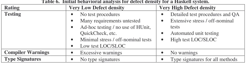
6.3 Step three: Perform behavioral analysis
The behavioral analysis for defect density in a Haskell system is shown in Table 6. While many aspects of this analysis are similar to that of STREW-J, there were specific concepts that were introduced specifically for a functional language.
Table 6. Initial behavioral analysis for defect density for a Haskell system.
Rating Very Low Defect density Very High Defect density
Testing • No test procedures
• Many requirements untested
• Ad-hoc testing / no use of HUnit, QuickCheck, etc.
• Minimal stress / off-nominal tests
• Low test LOC/SLOC
• Detailed test procedures and QA
• Extensive stress / off-nominal tests
• Automated unit testing
• High test LOC/SLOC
Compiler Warnings • Excessive warnings • No warnings
Type Signatures • No type signatures • Type signatures for all methods
6.4 Step four: Define relative significance
Based on our analysis of the literature and our experience with STREW-J, we determined that the metrics in STREW-H would behave in a similar manner to those in STREW-J. Thus, our initial reasoning was that testing effort would impact defect density the most, with type signatures next, and compiler warnings last.
6.5 Step five: Gather expert opinion
As we started to gather expert opinion on our model, we began to see how the two models would begin to move apart from one another. In January of 2004, interviews were conducted with 12 Haskell researchers at Galois Connections, Inc.12 and with members of the Programatica team13 at The OGI School of Science & Engineering at the Oregon Health and Science University (OGI/OHSU) to elicit expert opinion on the initial version of the STREW-H metric suite. We found that due to the nature of Haskell, more common Java errors
12 http://www.galois.com
such as type errors or null pointer exceptions did not exist. Even though versions of unit testing tools, such as HUnit (based on JUnit), existed, they were not used prevalently because most defects were discovered during system-level testing. Therefore, we determined that we required other types of metrics besides those mainly based on testing efforts to create our prediction. The suggested metrics from the Haskell experts included structural and testing concepts that are unique to functional languages. Using these suggestions, more background research was performed to validate the inclusion of these potential metrics in the STREW-H.
From gathered expert opinion and literature consulted, the following seven metrics were added to complete the STREW-H Version 0.1:
• monadic instances of code / source lines of code (M5), identified as a common source of problems in Haskell programs, provides information on likely problem areas;
• number of overlapping patterns / source lines of code (M6) shows the relative number of times that a pattern will never be reached because another pattern will overtake it, which is commonly a programmer error;
• number of incomplete patterns / source lines of code (M7) shows the relative number of patterns that will not complete because a case is not being covered;
• number of missing signatures / source lines of code (M8) shows the relative number of functions that do not have type signatures, a good programming technique;
• number of name shadowing / source lines of code (M9) shows the relative number of variables that have a variable of the same name in the same scope;
• number of unused binds / source lines of code (M10) shows the relative number of functions that were unused in the system;
• number of unused imports / source lines of code (M11) shows the relative number of imported modules that were unused in the system;
6.6 Step six: Formulate a-priori model
Similarly to STREW-J, the a-priori model for STREW-H was determined by applying the mathematical form of a regression analysis, which would be carried out once data from the project had been collected. This is shown in Equation 4.
Failures/KLOC = a + b*M1 + c*M2 + d*M3 + e*M4 + f*M5 + g* M6 + h*M7 + i*M8 + j*M9 + k*M10 + l*M11 (4)
Tools were also defined for gathering metrics. Various LOC counting tools, such as SLOCCount,14 and lexical analyzers, such as EditPlus,15 were used to the metrics. The metrics would be gathered on a static code
base at a specified point in the project. Specifically, snapshots of the code base would be taken at regular two-week intervals to assess development in-process.
6.7 Step seven: Gather project data
A subset of four metrics was gathered on seven different versions of the Glasgow Haskell Compiler (GHC) (Versions 4.08, 5.00.2, 5.02.2, 5.04, 5.04.3, 6.0, and 6.0.1). The system was around 200 KLOC in size. Only four metrics were gathered (M2 – M5) due to constraints on our ability to gather the other metrics at that time. GHC is hosted on SourceForge.net16 an open source development website. The website provides information on defects reported by version for a particular project. Defects had been reported for all versions included in this study, except for version 4.08, which was under development before the project was hosted on SourceForge. Defects from this version were taken from the GHC bugs mailing list archive17.
6.8 Step eight: Calibrate a-posteriori model
A multiple regression analysis18 was performed on these four metrics to determine if they were indicative of the number of defects that were found for each version. Six of the seven versions of GHC were randomly chosen to formulate the coefficients in the regression model, Equation 5. The regression equation was found to be:
Defects/KSLOC = .08 – .0762*(M2) + .0002*(M3) + .607*(M4) + .0113*(M5 ) (5)
The results of the study (p < .0451) show the model was statistically significant. Using this equation, the estimated defect density for the seventh version is 0.04 defects/KLOC, while the actual defect density was 0.07 defects/KLOC. The equation was fairly accurate in predicting the number of defects.
6.9 Step nine: Gather more data and refine model
The results of this study prompted further research with STREW-H. Based on the data we received regarding the various metrics and feedback from the Haskell experts, new metrics were added and old ones were refined to create a smaller, easier-to-use suite that still provided the same quality of information. This analysis prompted us to refine our metric suite to five metrics that cover both testing information and coding standards specific to the Haskell programming language. Our current version of STREW-H, Version 0.2 (Sherriff, Nagappan et al. 2005), is as follows:
• test lines of code / source lines of code (M1) includes HUnit, QuickCheck, and ad host tests and shows the general testing effort with respect to the size of the system;
16http://sourceforge.net/projects/ghc/
17http://www.haskell.org/mailman/listinfo/glasgow-haskell-bugs
• number of type signatures / number of methods in the system (M2) shows the ratio of methods that utilize type signatures, which is a good programming practice in Haskell;
• number of test cases / number of requirements (M3) includes HUnit, QuickCheck, and ad host tests and shows the general testing effort with regard to the scope of the system;
• pattern warnings / KLOC (M4) shows some of the most common errors in Haskell programming and includes common errors in the creation of recursive methods, such as incomplete patterns and overlapping patterns;
• monadic instances of code / KLOC (M5), identified as a source of problems in Haskell programs, provides information on likely problem areas.
6.10 Step seven: Gather project data – iteration 2
To validate STREW-H Version 0.2, we worked with Galois Connections, Inc., during the seven-month development of an ASN.1 compiler system (Sherriff, Nagappan et al. 2005). The project was a proof-of-concept ASN.1 compiler (about 20 KLOC) that could show that high-assurance, high-reliability software could be created using a functional language. During the course of the project, 20 in-process snapshots of the system were taken at one- or two-week intervals over the seven-month period. Also, logs were kept on the code base, indicating when changes needed to be made to the code to rectify defects that were discovered during the development process.
6.11 Step eight: Calibrate a-posteriori model – iteration 2
A multiple regression analysis19 was utilized to calibrate the model created with the five metrics of the STREW-H and the number of in-process defects that were corrected and logged in the versioning system by Galois. We calibrated the parametric model with 14 random in-process snapshots of the system and used this model to predict the remaining six snapshots’ defect densities. This data splitting was done five separate times with a different randomly-chosen set of 14 snapshots to help remove any bias. The analysis showed that future defect densities in the system could be predicted based on this historical data of the project with respect to the STREW-H metric suite.
The R2 values from the five models were as follows:
• 0.943 (F=26.304, p<0.0005);
• 0.930 (F=21.232, p<0.0005);
• 0.962 (F=25.206, p<0.0005);
• 0.949, (F=29.974, p<0.0005); and
• 0.967 (F=42.237, p<0.0005).
19 SPSS was used for the purpose of statistical analysis. SPSS does not provide statistical significance beyond three decimal
The results of the regression model showed that the STREW-H metrics are associated with the number of defects that were discovered and corrected during the development process. Using the parametric model, the defect density of the remaining six snapshots was predicted to be as shown in Figure 5. The graph in Figure 5 shows the closeness of the fit of the regression equation. Five of the six predictions were within 3 defects/KLOC, but one prediction was .8 defects/KLOC away from the actual value. We believe this occurred for this particular snapshot because it occurred during a time when new code development dropped and test code development increased. This change in their general weekly development methodology contributed to this outlier. For this model, the average absolute error is .299 and the average relative error is 14.091.
Case Number
6 5 4 3 2 1
D
ef
ec
ts
/
K
LO
C
2.5
2.0
1.5
1.0
.5
0.0
-.5
Actual Prediction LCL UCL
Figure 5: Actual vs. Estimated Defects/KLOC
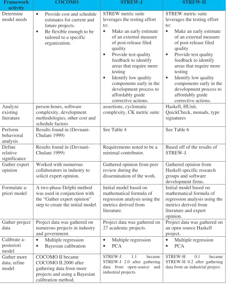
7 MODEL COMPARISON
Table 7. Model comparison. Framework
activity COCOMO STREW-J STREW-H
Determine
model needs • Provide cost and schedule estimates for current and future projects.
• Be flexible enough to be tailored to a specific organization.
STREW metric suite leverages the testing effort to:
• Make an early estimate of an external measure of post-release filed quality
• Provide test quality feedback to identify areas that require more testing
• Identify low quality components early in the development process to affordably guide corrective actions.
STREW metric suite leverages the testing effort to:
• Make an early estimate of an external measure of post-release filed quality
• Provide test quality feedback to identify areas that require more testing
• Identify low quality components early in the development process to affordably guide corrective actions. Analyze existing literature person-hours, software complexity, development methodologies, other cost and schedule factors
assertions, cyclomatic
complexity, CK metric suite Haskell, HUnit, QuickCheck, monads, type signatures
Perform behavioral analysis
Results found in
(Devnani-Chulani 1999) See Table 4 See Table 6
Define relative significance
Results found in
(Devnani-Chulani 1999) Requirements noted to be a minimal contributor. Based off of the results of STREW-J.
Gather expert
opinion Worked with numerous collaborators in industry to solicit expert opinion.
Gathered opinion from peer review during the
dissemination of the work.
Gathered opinion from Haskell-specific research groups and software development firms. Formulate
a-priori model A two-phase Delphi method was used in conjunction with the “Gather expert opinion” step to create the initial model.
Initial model based on mathematical formula of regression analysis using the metrics derived from literature.
Initial model based on mathematical formula of regression analysis using the metrics derived from literature and expert opinion.
Gather project
data Project data was gathered on numerous projects in industry and government.
Project data was gathered on
27 academic projects. Project data was gathered on an open source Haskell project.
Calibrate a-posteriori model
• Multiple regression
• Bayesian calibration •
Multiple regression
• PCA •
Multiple regression
• PCA
Gather more data; refine model
COCOMO II became COCOMO II.2000 after gathering data from more projects and using a Bayesian calibration method.
STREW-J 1.1 became STREW-J 2.0 after gathering data from open-source and industrial projects.
STREW-H 0.1 became STREW-H 0.2 after gathering data from an industrial project.
8 CONCLUSIONS
models in software engineering. We have also analyzed the creation three particular parametric models using this framework. Boehm’s COCOMO model has been built and refined over the course of more than 25 years to be an effective estimator of software project cost factors, and has been calibrated for use on numerous different types of software projects. The STREW-J and STREW-H models were created semi-concurrently, building off each other. The two models were calibrated to a much more narrow scope of systems, and certain companies in particular. They were shown to be effective estimators of software defect density.
While each follows the process in a different way, these three models demonstrate the utility of the nine-step process for building parametric models in software engineering. The process, while general enough to allow developers freedom in their approach, describes steps that can help direct model developers efforts so that important concepts are not overlooked. These steps are intended to be used as general guidelines, but the steps can and should be rearranged, combined, or omitted as necessary for a given project. For example, expert opinion was extremely important to COCOMO II in that it was used heavily in building the model through a Delphi process, and then it was used as the actual data for the model as well. STREW-H needed expert opinion to create the model since the model developer was not as familiar with the language. The model developer in STREW-J, however, only garnered expert opinion later in the process when validating the model. Each of these steps in the parametric modeling process provides different information for the model and can be emphasized in different ways. This flexibility in the process makes this parametric modeling process an effective tool for use in empirical software engineering.
9 ACKNOWLEGEMENTS
We would like to thank the members of the North Carolina State University Software Engineering Reading Group for reviewing initial drafts of this paper. The STREW-J work was funded in part by an IBM Eclipse Innovation Award. We would like to sincerely thank Galois Connections, Inc., and the Programatica Team at OGI/OHSU for their contributions to the STREW-H work. Additionally, this material is based upon work partially supported by the National Science Foundation under CAREER Grant No. 0346903. Any opinions, findings, and conclusions or recommendations expressed in this material are those of the author(s) and do not necessarily reflect the views of the National Science Foundation.
10 REFERENCES
Abts, C., B. W. Boehm, et al. 2000. COCOTS: a COTS software integration cost model. European Software Control and Metric Conference, Munich, Germany.
Basili, V., L. Briand, et al. 1996. "A Validation of Object Oriented Design Metrics as Quality Indicators." IEEE Transactions on Software Engineering 22(10): 751-761.
Basili, V. R., F. Shull, et al. 1999. "Building Knowledge Through Families of Experiments." IEEE Transactions on Software Engineering 25(4): 456 - 473.
Boehm, B. W. 1981. Software Engineering Economics. Englewood Cliffs, NJ, Prentice-Hall, Inc. Boehm, B. W. 2003. Building Parametric Models. International Advanced School of Empirical Software
Engineering, Rome, Italy.
Boehm, B. W., E. Horowitz, et al. 2000. Software Cost Estimation with COCOMO II. Upper Saddle River, NJ, Prentice Hall.