DOI: 10.1051/epjconf/20111204004 C
Owned by the authors, published by EDP Sciences, 2011
Probabilistic modelling of calcium leaching in a tunnel
for nuclear waste disposal
T. de Larrard
1,a, F. Benboudjema
1, J.-B. Colliat
1and J.-M. Torrenti
21LMT-ENS Cachan, CNRS/UMPC/PRES UniverSud Paris, France 2LCPC, Université Paris-Est, France
Abstract. This works aims at studying, through the Monte-Carlo method, the influence of the leaching kinetics parameters spatial variability on the lilfespan of a concrete structure. The considered structure is a tunnel for nuclear waste disposal. It is observed that the expected value for the lifespan estimated when considering the material spatial variability is significantly lower than the lifespan estimated with a single simulation considering uniform parameters fields, equal to the expected value for each parameter.
1. INTRODUCTION
Deep nuclear waste disposal facilities need to be studied over periods of one or more order of magnitude greater than those of classical civil engineering. This leads to consider some degradation phenomena that are most of the time not taken into account because of their slow kinetics. This is the case with calcium leaching for concrete structures exposed to water from the host rock in a deep underground disposal. Moreover, civil engineering constructions are naturally subjected to variability, from many origins: their dimensions, their construction processes, their exposure to several loadings... Among these variables, which influence the behaviour of the structure and, thus, its lifespan, some of them introduce a variability on the material characteristics, evolving with time and not necessary homogeneous in the whole structure, whereas some others create a variability on the loading itself, which the structure is subjected to.
The structure which we study is a tunnel for radioactive waste disposal. The objective is to confine the waste in a deep geological formation to protect the environment from the radionuclides they contain. This confinement has to be guaranteed over large time scales (up to several hundreds of thousands years) without requiring maintenance. The waste is contained in packages of metal or concrete, depending on the nature of the waste. These packages are arranged in cells, being disposal cavities in the rock. Under the hypothesis of reversible storage, packages are simply stored in the cells. If the option of underground disposal is finally adopted, the cells, and the tunnels leading to them, will be sealed.
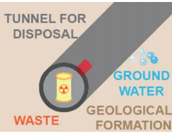
The structure we consider is one of these cells. For simplicity reasons and to ease the calculations, the considered geometry for the structure is very schematic: we simply consider a hollow cylinder, with an external radius of 8 m, and a thickness of 1 m. The disposal cell can reach a length of several hundreds meters. Figure1schematically represents the problem that we model. A tunnel for the waste packages disposal is dug in the soil, and a concrete wall protects the environment from the waste containers contained within the tunnel. The site water contained in the geological formation exposes the concrete tunnel to the risk of leaching. Even though this kind of degradation is very slow, it is to be considered as the required lifespan for such structures is several hundreds of thousands years.
ae-mail:
delarrard@lmt.ens-cachan.fr
Figure 1. Schematic representation of the considered structure: part of a tunnel for nuclear waste disposal exposed to ground water.
A numerical model for calcium leaching is developed and implemented in Finite Volumes simulation code. This model will be briefly presented in the first section of this paper. The second section introduces the statistical data we use to model the variability of our input parameters to model calcium leaching, being water porosity and coefficient of tortuosity. The last part is devoted to the investigation about the influence of this spatial variability on the lifespan of the tunnel. This study is performed by carrying out the Monte-Carlo method, which requires a large number of calculations. Moreover, as the accuracy of estimating the position of the degradation front depends on the refinement of the Finite Volumes mesh, it has been decided not to model the entire cell disposal, but only a part of it. The section considered in this application corresponds to an angular fraction of/12, as it appears on Fig.1. This is close to a block of 1 m high, wide and long.
Let us specify here that this problem is treated under a few strong assumptions, besides the geometric simplification of the structure:
• the influence of temperature is neglected, that is to say that the simulations are performed at constant temperature throughout the duration of the degradation (this assumption leads to overestimate the lifespan of the structure since the temperature might reach 60◦C for 10 years and 50◦C for 100 years according to the type of waste);
• any other interaction with the environment than leaching in pure water is not taken into account in modelling;
• leaching degradation is supposed to occur in pure water, whereas site water is actually loaded with different ions;
• no coupling with the mechanical behaviour of the structure is taken into account.
Finally, let us specify that the so-called lifespan of the structure in this study is the time necessary for the portlandite dissolution front to reach the inner wall of the tunnel.
2. CALCIUM LEACHING MODELLING
the solid phases of the material is modified. A new local equilibrium is then reached with the dissolution of solid phases [2].
Considering that the dissolution is instantaneous (local equilibrium) and that only calcium species are to be taken into account, the leaching of a cement paste can be described by the mass balance equation of calcium (1), as it was proposed by [3], whereSCais the solid calcium concentration,CCais
the liquid calcium concentration,Dis the calcium effective diffusivity in porous material andis the porosity. One can recognise the two main phenomena involved in the leaching process: on the one hand, the solid and liquid phases of calcium in the cement paste and in the porous solution are in chemical equilibrium; on the other hand, the ionic calcium species diffuse through the material porosity.
*(CCa)
*t = −div(D()grad(CCa))−
*SCa
*t . (1)
The non-linearity of the former equation is mainly due to the diffusivity which depends on the porosity, itself depending on the solid calcium concentration, and on the non-linearity betweenSCaandCCa. The
Finite Volume method [4] seems to be particularly accurate for our concern. Indeed it is well adapted to diffusion problems because its equations remain conservative. This is why a Finite Volume scheme has been chosen to pursue this study.
Considering the chemical laws of local equilibrium between the concentrations of liquid and solid calcium, every quantity appearing in (1) can be derived from the concentration of solid calcium, which reduces the problem to a single variableSCa. Considering concrete rather than cement paste leads to
the introduction of a tortuosity parameterstanding for the possible opposite effects of aggregates: on the one hand aggregates are areas where no diffusion occurs, but on the other hand they introduce an Interfacial Transition Zone where the diffusivity can increase due to a larger porosity of the ITZ in comparison with bulk cement paste [5]. This approach was successfully used by [6] and appears in (2) in order to express the diffusivity of calcium species through concrete depending on the cement paste porosity.
D()=D0ek. (2)
The implementation and validation of this numerical model are presented in [7]; this latter study also enhances that the most influential parameters on the leaching phenomenon kinetics are the porosity and the coefficient of tortuosity.
The main issue here is that porosity is a measurable parameter which can directly be observed for any considered concrete sample whereas the coefficient of tortuosity is a non-physical parameter and depends on the numerical model we chose. Therefore, an inverse analysis tool has to be developed so as to identify this coefficient from the observed experimental data, being the degradation depths at several terms of an accelerated leaching test. Among the numerous tools developed for inverse analysis, it has been chosen to use an Artificial Neural Network (ANN). It is used as follows: the input data are the values measured for the porosity and the degradation depths for each sample, and a mean value of temperature for each period of degradation. The output data is an identified value of coefficient of tortuosity.
3. MONTE-CARLO INTEGRATION AND RANDOM FIELDS GENERATION
As explained above, the key step to carry out the Monte-Carlo integration is to generate an important number of realisations of the porosity and the coefficient of tortuosity random fields. Although these realisations must be independent, they are all spatially correlated and the synthesis process is not trivial. A very efficient way to achieve it is to employ the Karhunen-Loève expansion as explained by [9]. The key idea of the Karhunen-Loève expansion is to expand any second-order random fieldf(x, ) into a serie (3). Each term of this serie is a product of two terms, the first one depending on the spatial variablexand the second one depending on the stochastic variable. Thus, the main feature of such a decomposition is the separation of variable.
f(x,)=f¯(x)+ +∞
i=0
ii(x)i(). (3)
The first term of (3) is the expected value of the random field. The stochastic dependency appears through the random variables i, while the spatial dependency is introduced through the covariance kernel eigenmodes (i,i), where the i are the eigenvalues and the i are the corresponding
eigenvectors. Moreover, it is worth noting that the random variables i form a set of orthonormal variables. Finally, dealing with Gaussian random fields, thei are Gaussian random variables as well and, being uncorrelated, they are independent. Thus (3) provides a very efficient way to synthesise correlated random fields realisations, independent from one another.
Considering the generalised eigenvalues problem, we are interested in determining the largest eigenvalues. A convenient way to achieve this is to perform a Finite Elements discretisation of the problem (see [10]), leading to the discrete generalised eigenvalues problem (4), whereMis the mass matrix with a unitary mass density andCis the covariance matrix.
MCM=M. (4)
This numerical problem is very alike to eigenvalues problems encountered in structural dynamics. Therefore, a Finite Element code (FEAP) has been used to determine the Karhunen-Loève eigenmodes by re-using the FEAP routines with the appropriate matrixes. It is worth noting that, even thoughMis a sparse matrix - due to the FE properties - the covariance matrixCis a full one. This point may lead to some difficulties linked to disposal and memory requirements.
Once a set of the largest eigenvalues, as well as the corresponding eigenvectors, has been determined, the truncated Karhunen-Loève expansion enables the approximation (5) for any second-order random field. In this approximationmis the number of modes which are considered and it can be shown that (5) is optimal alongm[11,12]. Assuming the random field to be Gaussian, the random variablesi are
normally distributed with zero expectation and variance equal to one. This series truncation introduces an error in the field approximation, which decreases whenmincreases. The theoretical background of the Karhunen-Loève expansion can be carried out to calculate the eigenmodes of the covariance kernel. Once these modes are in hands, the expansion can be exploited as many times as necessary to compute the random fields realisations required for the Monte-Carlo Method.
ij =¯i+ m
k=1
kkikj. (5)
4. VARIABILITY OF POROSITY AND COEFFICIENT OF TORTUOSITY
two different kinds of concrete mix design, the first one being a high-performance concrete with fly ash and the second one being an ordinary concrete.
For each construction site and so for each concrete formulation, 40 batches are characterised through several tests performed in laboratory (such as compressive and splitting tensile strength, static and dynamic Young modulus, electrical resistivity, etc.). All the concrete samples necessary for the tests are directly provided by the construction site to the involved laboratories. The concrete samples are protected from drying thanks to plastic bags. Then they are stored in saturated lime water. The concrete specimens are one year old at the beginning of each test. This campaign aims at acquiring statistical data on the material characteristics and investigating the variability of these characteristics within several batches of a same formulation and also between different concrete mix design. The porosity measurement and the accelerated leaching tests were performed in LMT Cachan. The whole experimental campaign is presented in detail in [14]. For this study, only the results on the A1 concrete are considered, because the following numerical investigation is based on the experimental observations for this concrete mix design.
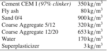
The so-called A1 concrete is the high-performance concrete with fly ash used for the A84 highway tunnel near Paris (France). Table1 presents the concrete mix design used for this building operation. In Table2, the basic physical characteristics of this material are summarised. In this table appear the average values experimentally observed during the APPLET campaign for the electrical resistivityel,
the volumic weigth, the compressive strength 28 days after castingF c28 and the compressive strength after one year in saturated lime solution storageF c365, the tensile splitting strengthFcand the Young modulusE.
Table 1. Concrete mix design for A1 building operation.
Cement CEM I(97% clinker) 350 kg/m3
Fly ash 80 kg/m3
Sand 0/4 900 kg/m3
Coarse Aggregate 5/12 320 kg/m3
Coarse Aggregate 12/20 653 kg/m3
Water 170 kg/m3
Superplasticizer 3 kg/m3
Table 2. Basic physical characteristics observed for A1 concrete.
el 351 .m
2.25 g.cm−3
F c28 57.9 MPa
F c365 83.8 MPa
F t 4.9 MPa
E 46.7 GPa
As mentioned above, one of the main parameters involved in the leaching process is the water porosity measured on sound concrete. Each batch of concrete studied in the project is characterised by the measurement of its water porosity, which is calculated on the basis of three mass measurements: two performed on a saturated slice of concrete (full atmospheric and hydrostatic weight,MairandMwater)
and one performed on the dried slice (105◦C in a furnace till constant mass,Mdry) [15], according to
equation (6).
=100 Mair−Mdry
Mair−Mwater
For each batch, a concrete sample is devoted to a leaching test. Leaching in pure water usually presents a very slow kinetic and one of the most common ways to accelerate it is to use ammonium nitrate solution [17,18]. Calcium concentration increases significantly (from 22 mol/m3to 2700 mol/m3 for
a concentration of 6 mol/L of ammonium nitrate), which accelerates the degradation kinetics at least by a factor 100. At fixed dates (28, 56, 98 and 210 days), the degradation depth is revealed with phenolphthalein.
Actually, it seems that the degradation depth revealed with phenolphthalein is not exactly the position of the portlandite dissolution front [16], but the ratio between both is not completely acknowledged: it does not seem constant in time neither with different degradation conditions. Therefore, it will be considered in this study that the degradation depth is the one revealed with phenolphthalein.
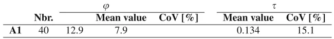
For each concrete sample, the coefficient of tortuosity is identified with the Artificial Neural Network introduced in Section2. Thanks to this experimental and identification campaign, one can quantify the variability observed between several batches of the same concrete mix design on a building site for porosity and coefficient of tortuosity. These results are presented for the A1 concrete of the APPLET project in Table3.
Table 3. Water porosity and coefficient of tortuosity: number of tested samples, mean value and coefficient of variation for A1 concrete of the APPLET project.
Nbr. Mean value CoV [%] Mean value CoV [%]
A1 40 12.9 7.9 0.134 15.1
If the experimental campaign results presented above allow us to propose a quantification of the variability for both porosity and coefficient of tortuosity (especially in terms of average and standard deviation), they do not, however, provide any information about the spatial correlation for these fields. Therefore, an experimental wall was cast, and samples were taken along two horizontal lines and one horizontal line. This wall was made with a construction joint at half height, so that each horizontal line is in a different batch. The samples are cores of 10 cm large and 30 cm high. However, the two batches were cast the same day, so there is very few difference between the two batches and the experimental results shall be regarded as from one batch only. On each sample, water porosity and resistance to an accelerated leaching test are measured, following the same protocol as presented above. So we can identify, for each sample, the water porosityand the coefficient of tortuosity.
In our case, we assume that our random fields (porosity and coefficient of tortuosity) are spatially correlated according to the covariance function given in equation (7) whereC(x,y) is the covariance between two points,xandy, and2is the random field variance, whileLcis a scalar parameter called
correlation length. This latter parameter reflects the importance of the field spatial correlation: the higher the value, the stronger the field is correlated, so that for an infinite correlation length the field would tend to be uniform.
C(x,y)=2exp
−x− y2
L2 C
. (7)
This covariance function has the advantage of being differentiable at 0. For better understanding, let us recall that the covariance is an indicator of the degree of dependence between two variables: if the covariance of two variables is zero, they are independent from one another, that is to say that their respective variations are independent. Thus the parameterLctranslates the random fields spatial
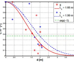
Figure 2.Correlation lengths identification from the variograms for the two considered random variables on the horizontal line in batch 2.
geometry and to identify the correlation length. Indeed, by definition, the covariance between two points xandyfor a random variable respectively equal toXandY, written asC(x,y)=E[(X−E[X])(Y − E[Y])], where the expected value of a random variable is denotedE.
However, if one has only a single realisation of the considered random field (as it is the case here: one experimental wall), it is possible to determine the covariance from a variogram. For a given random variable, the value of the variogram at distanced is the half-mean square differences of its realisations on the set of points spaced ofd. For a given random field, if covariance is defined, its value for a distance
dis equal to the difference between the covariance at 0 and the value of the variogram atd. Covariance at 0 simply is the variance. Since the variogram can be determined from a single realisation of the field, discrete values of the covariance can be deduced. Then we identify the value of the parameterLcin the
covariance function (7).
To conclude, Fig. 2 shows the covariance values obtained from the measurements on the wall compared to the corresponding covariance function. One can plot the normalised covariance (with regards to the variance for each variable: porosity and coefficient of tortuosity) on the horizontal line in batch 2 for instance (see Fig.1Fig.2).
It is observed in all cases that the correlation lengths are by the order of magnitude of one meter, and are similar for all three studied lines, whatever the considered variable. However, since the accordance between the proposed correlation function and the variogram values observed for the two variables is only relatively satisfactory, and given the low number of measurement points from which the study was conducted and the small size of the experimental wall (with regards to the scale of an entire structure), these values of correlation lengths (summarized in Table.4) should be considered with caution. Table 4. Identified correlation lengths for porosity and coefficient of tortuosity on the experimental wall.
Lc[m]
Horizontal line, batch 1 0.36 1.21 Horizontal line, batch 2 1.66 1.99
Vertical line 1.97 2.33
5. RESULTS AND ANALYSIS
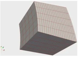
Figure 3. Finite Volumes mesh for the modelled part of the tunnel.
a. Lifespans distribution b. Cumulative distribution
Figure 4. Fitting of a generalised extreme value distribution law parameters in the case Lc=0.5 m.
. These two variables are assumed independent. Three values of correlation lengths are tested, by the order of magnitude identified on the experimental wall: 0.5 m, 1 m and 2 m.
The lifespans estimated by taking into account the input parameters variability are to be considered with respect to a reference value which is given by a deterministic simulation, that is to say, a simulation with uniform fields of porosity and coefficient of tortuosity, equal to the expected value of these parameters. Indeed, the expected value for any output of a problem is not equal to the output of the same problem considered with the expected values of its input parameters. Figure 3shows the mesh chosen for these simulations. The sides of the element, which are not exposed to site water, are assumed to be subjected to a null flux. There are 10 control volumes along the length of the structure (parallel to a generatrix of the cylinder), 10 orthoradial volumes and 20 volumes in the thickness.
The reference simulation is conducted with uniform fields of porosity and coefficient of tortuosity, being respectively equal to 12.9% and 0.134. The result in this case is the reference value for the lifespan of the tunnel: 254,000 years
Let us observe the results in the case of a correlation length of 0.5 m. Figure4shows the results of the Monte Carlo simulations and compares them with the result of the reference simulation (Figure4(a)). Figure 1 represents the lifespans distribution and it is to be noticed that the expected value for the probabilistic lifespan is significantly lower than the reference value (227,554 years vs. 254,000 years). In this figure, one can also observe a generalised extreme value distribution law, which is the statistical law which reproduces better the results distribution.
a. Lc= 1.0 m b. Lc= 2.0 m
Figure 5. Comparison between lifespans cumulative distribution and log-normal, logistic and generalised extreme value cumulative distribution laws.
structures have a lifetime of less than 198,760 years, to be compared to the 254,000 years of the reference simulation, which stands for a difference of almost 22%.
It is verified that in all cases of correlation length, the expected value for simulations taking into account the input fields variability is significantly lower than the reference value of lifespan: 245,648 years and 225,883 years respectively for a correlation length of 1 m and 2 m, instead of 254,000 years for uniform fields.
It also is noticeable that the coefficient of variation increases with the correlation length: 10.6% for Lc=50 cm, 12.0% forLc=1 m and 16.4% forLc=2 m. This increase in the coefficient of variation
with the correlation length is mainly due to the fact that a large correlation length (in the latter case the correlation length is two times greater than the tunnel thickness) implies the existence of "extreme cases" among the realisations of the random field, that is to say uniformly low (or on the contrary high) realisations, which would lead to penetration velocity of the degradation front substantially smaller (or larger) compared to the real uniform case with the expected values of porosity and coefficient of tortuosity.
For each case of correlation lengths, 3 distribution laws are fitted on the results distribution: log-normal, logistic and generalised extreme value distribution law. All three laws reveal to be quite relevant to model the results distribution. The values of the statistical laws parameters, identified on the simulation results for the three studied cases of correlation lengths, are listed in Table5. Figure5 compares the simulation results distribution for different values of correlation length with the three distribution models (log-normal, logistic and generalised extreme value).
Table 5. Identified values of the distribution laws parameters.
Log-normal distribution Logistic distribution Generalised extreme value distribution
Lc=0.5 m 12.33 0.106 225,142 11,757 217,159 17,105 0.036
Lc=1.0 m 12.40 0.119 245,842 15,837 234,648 30,045 -0.237
Lc=2.0 m 12.31 0.163 224,058 21,373 210,224 32,583 -0.114
lifespan: 90% of the structures have a lifespan of less than 254,000 years for Lc=0.5 m, 60% for Lc=1 m and 75% for Lc=2 m.
It is not clear from this study what the influence of the correlation length on the expected value for the lifespan is, provided it is more important for a correlation length of 1 m than for 50 cm or 2 m. The direct conclusions from this study are firstly that the lifespan variability increases with the correlation length, and secondly that in all the cases treated here, the expected value is less than the reference lifespan (estimated by a deterministic calculation based on the expected values of the input parameters). Also note that only three correlation lengths have been tested, relatively close to one another, and by the same order of magnitude as the size of the studied structure.
Similarly, if one considers for each case the lifespan corresponding to the 5% fractile, it appears that: • for a 50 cm correlation length: 5% of the structures have a shorter lifespan than 198,760 years (i.e.
22% lower than the reference value for lifespan);
• for a 1 m correlation length: 5% of the structures have a shorter lifespan than 199,210 years (i.e. 22% lower than the reference value for lifespan);
• for a 2 m correlation length: 5% of the structures have a shorter lifespan than 172,150 years (i.e. 32% lower than the reference value for lifespan).
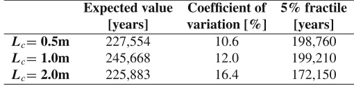
All statistical information derived from the distributions of the Monte-Carlo simulations results for the three tested values of correlation length is presented in Table6.
Table 6. Synthesis of the Monte-Carlo simulations results for the three studied values of correlation length.
Expected value Coefficient of 5% fractile [years] variation [%] [years]
Lc=0.5m 227,554 10.6 198,760
Lc=1.0m 245,668 12.0 199,210
Lc=2.0m 225,883 16.4 172,150
6. CONCLUSIONS
The purpose of this study was to observe the effect of the spatial variability of material properties (porosity and coefficient of tortuosity) on propagation velocity of the dissolution front of portlandite in a concrete structure. It appears that a simulation considering uniform fields, equal to the average value of experimental observations for the concerned parameters, leads to estimate a lifetime greater than at least 60% of the structures simulated by taking into account the observed variability. In addition, more than 5% of the structures have a lifespan lower than 80% of the lifespan estimated with uniform fields. The main conclusion to be drawn from this study about the influence of the correlation length is that the output of interest variability increases with the correlation length. This is a consequence of the fact that considering a large correlation length leads to the appearance of “extreme cases” in the realisations of the random fields. However, this study is rather limited, since only three values of correlation length have been tested, and all by the same order of magnitude (but corresponding to the observations of the APPLET experimental campaign). In addition, another limit to this study is the size of the structure under consideration: the interest of simulations with very large correlation lengths compared to the largest dimension of the structure is somewhat restricted (such simulations get closer to simulations considering a scalar variable instead of a random field).
References
[1] Torrenti J.-M., Didry O., Ollivier J.-P., Plas F.,La dégradation des bétons – couplage fissuration-dégradation chimique(Hermès, 1999)
[2] Adenot F., Durabilité du béton : caractérisation et modélisation des processus physiques et chimiques de dégradation du ciment(PhD Thesis, Université d’Orléans, France, 1992)
[3] Buil M., Revertégat E., Oliver J., A Model of the Attack of Pure Water or Undersaturated Lime Solutions on Cement, vol. 2nd, pp. 227-241 (American Society for Testing and Materials,
Philadelphia, 1992)
[4] Mainguy M., Tognazzi C., Torrenti J.-M., Adenot F.,Modelling of leaching in pure cement paste and mortar, Cement and Concrete Research,30, pp. 83-90 (2000)
[5] Ollivier J.-P., Maso J.-C., Bourdette B.,Interfacial transition zone in concrete, Advanced Cement Based Materials,2, pp. 30-38 (1995)
[6] Nguyen V.-H., Nedjar B., Colina H., Torrenti J.-M., A separation of scales homogenisation analysis for the modelling of calcium leaching in concrete, Computer Methods in Applied Mechanics and Engineering,195, pp. 7196-7210 (2006)
[7] de Larrard T., Benboudjema F., Colliat J.-B., Torrenti J.-M., Deleruyelle F., Concrete calcium leaching at variable temperature: experimental data and numerical model inverse identification, Computational Materials Science,49, pp. 35-45 (2010)
[8] Caflisch R. E.,Monte Carlo and Quasi-Monte Carlo Methods, Acta Numerica,7, pp. 1-49 (1998) [9] Spanos P. D., Ghanem R. G.,Stochastic finite element, a spectral approach(Dover Publication,
2002)
[10] Keese A.,Numerical solution of systems with uncertainties – a general purpose framework for stochastic finite elements(PhD Thesis, Technischen Universitat Braunschweig, Germany, 2003) [11] Karhunen K., Über lineare Methoden in des Wahrscheinlichkeitrechnung, ANN. Acad. Sci.
Fennicae, Ser. Al. Math.-Phys.,37, pp. 1-79 (1947)
[12] Loève M.,Probability theory, vol. II of Graduate Texts in Mathematics, 4thedn (Springer-Verlag, 1978)
[13] Poyet S., Torrenti J.-M., Caractérisation de la variabilité des performances des bétons. Application à la durabilité des structures (groupe de travail APPLET), Annales du BTP, 2-3, pp. 6-12 (2010)
[14] de Larrard T., Etude probabiliste des propriétés du béton. Applications aux enceintes de confinement et au stockage des déchets radioactifs(PhD Thesis, ENS Cachan, France, 2010) [15] AFPC-AFREM,Durabilité des bétons – Méthodes recommandées pour la mesure des grandeurs
associées à la durabilité (Compte-rendu des Journées Techniques AFPC-AFREM, Toulouse, France, 1997)
[16] Le Bellégo C., Couplage chimie-mécanique dans les structure en béton attaquées par l’eau : étude expérimentale et analyse numérique(PhD Thesis, ENS Cachan, France, 2001)
[17] Lea F. M.,The action of ammonium salts on concrete, Magazine of concrete research,52, pp. 115-116 (1965)