Article
Dynamic Complexity Measures: definition and
calculation
JoséRobertoC.Piqueira
Escola Politécnica da Universidade de São Paulo
Departamento de Engenharia de Telecomunições e Controle Av. Prof. Luciano Gualberto, travessa 3, n. 158
05508-900, São Paulo, Brasil
* [email protected]; Tel.: +55-11-3091-5221
Abstract: This work is a generalization of the López-Ruiz, Mancini and Calbet (LMC); and Shiner,
1
Davison and Landsberg (SDL) complexity measures, considering that the state of a system or process 2
is represented by a dynamical variable during a certain time interval. As the two complexity 3
measures are based on the calculation of informational entropy, an equivalent information source 4
is defined and, as time passes, the individual information associated to the measured parameter is 5
the seed to calculate instantaneous LMC and SDL measures. To show how the methodology works, 6
an example with economic data is presented. 7
Keywords: Complexity; disequilibrium; equilibrium; individual information; informational
8
entropy. 9
Key contribution:LMC and SDL complexity measures are generalized for temporal series
10
Calculations are based on the construction of an informational source 11
LMC and SDL measures present the same qualitative dynamics 12
Partition of the range interval depends on the observation time interval 13
1. Introduction
14
The word complexity, in the common sense meaning, represents systems that are difficult to 15
describe, design or understand. However, since Kolmogorov presented the concept of computational 16
complexity [7], new ideas have been associated to this word, mainly concerning life sciences [1], 17
relating complexity with information [5]. 18
As a consequence, complexity started to be related to open systems and to the emergence 19
of unexpected behaviors, due to nonlinearities [11,13] and, concerning system theory [25], a new 20
meaning was carved, considering that complexity is half way of the equilibrium and disequilibrium 21
[6]. 22
Considering this idea, López-Ruiz, Mancini and Calbet proposed, in a seminal paper [8], the 23
LMC complexity measure by using the informational entropy [22] to evaluate equilibrium, and a 24
quadratic deviation from the uniform distribution to evaluate disequilibrium. 25
However, there are some criticisms about LMC measure, considering that it is inaccurate for 26
some classes of systems obeying Markovian chains and can not be considered an extensive variable. 27
Feldman and Crutchfield [4] proposed a correction for the disequilibrium term, replacing it by the 28
relative entropy with respect to the uniform distribution. 29
Following this line, Shiner, Davison and Landsberg proposed another modification of the LMC 30
measure, replacing the disequilibrium term by the complement of the equilibrium term. This measure 31
is called SDL [23] and presents results qualitatively similar to the obtained by using LMC, for the 32
majority of usual statistical distributions [15]. 33
The main restriction to LMC and SDL complexity measures is due to Crutchfield, Feldman and 34
Shalizi, as they argue that an equilibrium system can be structurally complex [3], but this problem 35
could be solved weighting order and disorder, according to the specific problem to be analyzed [16]. 36
Since the early 2000’s, the idea of adapting LMC and SDL to dynamical systems was successfully 37
applied to different types of time evolution problems: sleep-awake cycle [21], bird songs [24], 38
neural plasticity [10,14], interactions between species in ecological systems [1,19], physiognomies of 39
landscapes [9], economical series [12,20], spread depression [18] and quantum information [2,17]. 40
With these ideas in mind, this article presents a systematization of the methodology used in the 41
referred papers, based on LMC and SDL measures, to be applied to temporal series, by defining and 42
calculating dynamical complexity measures. 43
The procedure, applied to a temporal series representing some organizational or dynamical 44
aspect of a system, provides hints regarding the evolution of its complexity. 45
As the LMC and SDL dynamical measures are based on informational entropy [12], the first task, 46
described in the next section, is to define an alphabet source, associating a probability distribution to 47
the possible system states. 48
Following the definition of the probability distribution, a new section defines how dynamical 49
LMC and SDL measures can be calculated at each time, based on the individual information 50
associated to the system state at this time, generating temporal series for LMC and SDL measures. 51
To illustrate the calculation procedure, an example related to an economical time series is 52
presented and, in the same section, a practical discussion about how to divide the range of the values 53
assumed by the system state is presented. 54
The work is closed with a conclusion section, emphasizing that the calculations presented can be 55
applied to any kind of temporal real numbers series. 56
2. Defining source and probability distribution for a temporal series
57
Considering the Shannon’s model [22] for an information source, a time seriesx(n)is considered 58
to be a function of the integers into a real interval, i.e.,x(n) : Z+ → (a,b), associating to each time 59
t0+nTa real number belonging to(a,b), witht0>0 being the initial instant andT>0 an arbitrary
60
period, depending on the data availability. 61
The first step is to divide the interval(a,b)into N sub-intervals. For the sake of simplicity, N is 62
chosen equal to 2k,k∈Z+. 63
At this point, it could be asked how to choose N, as there is a compromise between precision 64
(high values of N) and speed of calculation (low values of N). This question will not be addressed 65
theoretically; however in the example section, practical hints about the choice will be presented. 66
Consequently, the source’s alphabet is defined by the intervalsAi,i=1, ...,N, withSNi=1= (a,b)
67
andAiTAj=φ,∀i6= j. 68
Then, a time interval defined by a given n must be chosen, and for the time sequence 69
t0,t0+T, ...t0+nTthe values of the variablex(n)must be read and associated to the intervals Ai, 70
containing the respective value. 71
Therefore, for the whole sett0,t0+T, ...t0+nT, each intervalAi is associated tox(n)a certain 72
number of timesni, which defines a relative frequency pi = nn+i1, taken as a probability, associated
73
each intervalAi. 74
Following the definition, for each sub-interval Ai ∈ (a,b), its individual contribution to the 75
whole information entropy is given by:Si=−pilog2pi; and the maximum value of the informational 76
entropy for the whole source,Smax=log2N=k, can be calculated [22].
3. Dynamical LMC and SDL
78
As the source alphabet and individual information were defined, the instantaneous values of 79
x(n) are associated to the respective Si, allowing the calculation of the instantaneous value of the 80
equilibrium (disorder) term: 81
∆(n) = Si
k. (1)
Combining (1) with the different definitions of the disequilibrium (order) terms, dynamical LMC 82
and SDL measures are defined. 83
3.1. LMC dynamical measure 84
As indicated by López-Ruiz, Mancini and Calbet [8], the dynamic disequilibrium (order) term 85
can be calculated as the quadratic deviation of the source probability distribution from the uniform 86
distribution and, consequently, the individual contribution of the intervalAiis: 87
D(n) = (pi−1/N)2. (2)
Extending the definition of LMC measure, dynamical LMC, calculated int0+nT, is given by:
88
CLMC(n) =∆(n).D(n). (3)
3.2. SDL dynamical measure 89
As proposed by Shiner, Davison and Landsberg [23], the dynamic disequilibrium (order) term 90
can be calculated as the complement of the dynamic equilibrium term: 91
D(n) = (1−∆(n)) (4)
Extending the definition of SDL measure, dynamical SDL, calculated int0+nT, is given by:
92
CSDL(n) =∆(n).D(n). (5)
4. Applying the method: practical hints
93
In this section, the economic series relative to the conversion of currencies studied in [12,20] is 94
taken as an example, concerning only to the methodological point of view, without any economic 95
conjecture about the results. 96
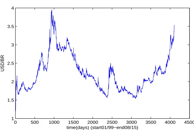
The daily conversion rate dollar to Brazilian real (USD/BR) temporal series, from January 1999 to 97
September of 2015, shown in Fig.1 [12,20] represents the value ofx(n), which complexity is analyzed. 98
Consequently, the interval(a,b)related to the excursion ofxis(1.207; 4.178). It is divided into 99
8(k = 3), 16(k = 4), 32(k = 5)and 64(k = 6)subintervals to build the sources and the respective 100
probability distributions. 101
Based on these probability distributions,CLMC(n)andCSDL(n)are calculated and plotted giving 102
an idea about how measure choice and interval division affects the results. 103
4.1. Equivalence between LMC and SDL 104
Dividing the range ofx(n)into 8 parts, the results of the calculation ofCLMC(n)andCSDL(n) 105
measures are shown in Fig. 2a and 2b, respectively. 106
As Fig. 2a and 2b show, in spite of the numerical differences, the time evolution ofCLMC(n)and 107
CSDL(n)are qualitatively the same and represented by very similar curves, in the eight-part division 108
0 500 1000 1500 2000 2500 3000 3500 4000 4500 1
1.5 2 2.5 3 3.5 4
time(days) (start01/99−end08/15)
USD/BR
Figure 1.USA Dollar-Brazilian Real exchanging rate
0 500 1000 1500 2000 2500 3000 3500 4000 4500 0
1 2
x 10−4
LMC
time(days) (01/04/1999 to 09/22/2016)
(a) LMC
0 500 1000 1500 2000 2500 3000 3500 4000 4500 0
1 2 3 4 5 6 7 8 9x 10
−3
SDL
time(days)(01/04/1999 to 09/22/2016)
(b) SDL
0 500 1000 1500 2000 2500 3000 3500 4000 4500 0
0.5 1 1.5 2 2.5 3 3.5 4 4.5x 10
−5
LMC
time(days)(01/04/1999 t0 09/22/2016)
(a) LMC
0 500 1000 1500 2000 2500 3000 3500 4000 4500 0
0.5 1 1.5 2 2.5 3 3.5 4 4.5x 10
−3
SDL
time(days)(01/04/1999 to 09/22/2016)
(b) SDL
Figure 3.Temporal evolution of complexity (16-part division)
0 500 1000 1500 2000 2500 3000 3500 4000 4500 0
1 2 3 4 5 6 7 8x 10
−6
time(days)(01/04/1999 to 09/22/2016)
LMC
(a) 32-part partition
0 500 1000 1500 2000 2500 3000 3500 4000 4500 0
0.2 0.4 0.6 0.8 1 1.2x 10
−6
LMC
time(days)(01/04/199 to 09/22/2016)
(b) 64-part partition
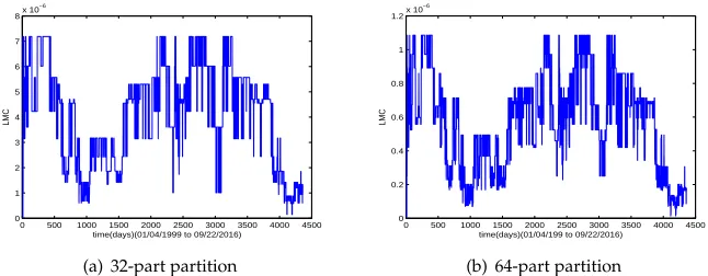
Figure 4.Temporal evolution of LMC complexity
If the range ofx(n)is divided into 16 parts, Fig. 3a and 3b show the results for CLMC(n)and 110
CSDL(n). 111
It can be observed that, in this case (sixteen-division case),CLMC(n)andCSDL(n)differ only by 112
a scale factor, with the same qualitative time evolution. 113
Comparing Fig. 2a and 3a,CLMC(n)for different range partitions, the whole qualitative aspects 114
of the curves are the same and by increasing the number of divisions, the dynamical range of the 115
measures changes, implying some rapid oscillatory variations, similar to noise. 116
Comparing Fig. 2b and 3b,CSDL(n)for different range partitions, the whole qualitative aspects 117
of the curves are the same and the noisy aspect due to the increasing number of interval divisions is 118
maintained. 119
Consequently, from now on, only LMC measure will be analyzed, since SDL presents the same 120
qualitative dynamical behavior and partition sensitivity. 121
4.2. Range interval partition 122
By increasing the number of intervals of thex(n) and recalculatingCLMC(n), the result for a 123
thirty-two partition is shown in Fig. 4a and, for a sixty-four partition, in Fig. 4b. 124
By analyzing the results from figures 2a, 3a, 4a and 4b it could be observed that by increasing 125
the number of intervals, the maximum value of CLMC(n) decreases improving the precision but, 126
apparently, for this long series the temporal evolution ofCLMC(n)maintains its qualitative behavior 127
mixing noise with accuracy. 128
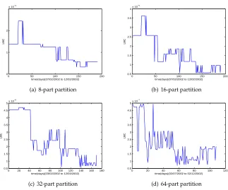
Attempting to be more precise about how the range interval partition, theCLMC(n)is calculated 129
for the several partitions, but considering a shorter time period for the data. The interval between July 130
and December of 2002 is chosen, because, as explained in [12], it is critical concerning the conversion 131
0 50 100 150 200 0
1 2
x 10−4
LMC
time(days)(07/02/2002 to 12/02/2002)
(a) 8-part partition
0 50 100 150 200 0.5
1 1.5 2 2.5 3 3.5
4x 10
−5
time(days)(07/02/2002 to 12/02/2002)
LMC
(b) 16-part partition
0 20 40 60 80 100 120 140 160 180 0.5
1 1.5 2 2.5 3 3.5 4 4.5
5x 10
−6
LMC
time(days)(03/02/2002 to 12/03/2002)
(c) 32-part partition
0 20 40 60 80 100 120 0.5
1 1.5 2 2.5 3 3.5 4 4.5
5x 10
−7
LMC
time(days)(02/07/2002 to 02/12/2002)
(d) 64-part partition
Figure 5.LMC temporal evolution for shorter time intervals
Figures 5a, 5b, 5c, 5d show the LMC dynamical measure calculated, for the initial set of data, 133
with the range interval divided into 8, 16, 32 and 64 parts, respectively. 134
It can be observed from these results that, for shorter intervals, the general qualitative 135
characteristics of the time evolution appear, independently on the partition. However, as the number 136
of sub-intervals increases, the instantaneous numerical values change but the precision increases, 137
allowing more accurate analysis. 138
5. Conclusions
139
A methodology for calculating LMC and SDL dynamical complexity was developed, starting 140
with the construction of a source and a probability distribution, for any temporal series. 141
It was observed that LMC and SDL measures, in spite of presenting different numerical results, 142
have very similar temporal evolution, related to the variablex(n). 143
A point that is always object of discussion is the range interval partition. The choice of the 144
number of sub-intervals is a matter of experience. 145
Long time intervals are not so sensitive to the increase of the number of divisions; however, for 146
short time intervals, increasing the number of divisions provokes a precision improvement, in spite 147
of the introduction of an apparent noise. 148
149
1. M. Anand & L. Orlóci, “Complexity in plant communities: the notion of quantification",Journal of Theoretical 150
Biology,179, (1996) pp. 179-186.
151
2. Y. C. Campbell-Borges & J. R. C. Piqueira, “Complexity Measure: A Quantum Information Approach",
152
International Journal of Quantum Information,10, (2012), pp. 1250047-1-1250047-19.
153
3. J. P. Crutchfield, D. P. Feldman & C. R. Shalizi, “Comment I on “Simple measure for complexity"",Physical 154
Review E,62, (2000), 2996.
155
4. D; P. Feldman & J. P. Crutchfield, “Measures of statistical complexity: Why?",Physics Letters A.238, (1998)
156
pp. 244-252.
5. H. Haken,Information and Self-Organization, (2000), Springer-Verlag: Berlin, Germany.
158
6. K. Kaneko & I. Tsuda,Complex Systems: chaos and beyond, (2001), Springer Verlag: Berlin, Germany.
159
7. A.N. Kolmogorov, “Three approaches to the definition of the concept “quantity of information””,Problemy 160
Peredachi Informatsii,1(1965) pp. 3-11.
161
8. R. López-Ruiz, H. L. Mancini and X. Calbet, “A statistical measure of complexity”,Physics Letters A,209 162
(1995) pp. 321-326.
163
9. S. H. V. L. de Mattos, L. E. Vicente, A. Perez Filho, J. R. C. Piqueira, “Contributions of the complexity
164
paradigm to the understanding of Cerrado’s organization and dynamics",Anais da Academia Brasileira de 165
Ciências,88(4), (2016), pp. 2417-2427.
166
10. M. Mazza, M. Pinho, J. R. C. Piqueira & A. C. Roque, “A Dynamical Model of Fast Cortical Reorganization",
167
Journal of Computational Neuroscience,16(2),(2004), pp. 177-201.
168
11. E. Morin,On complexity, (2008), Hampton Press: New York, USA.
169
12. L. P. D. Mortoza & J. R. C. Piqueira, “Measuring complexity in Brazilian economic crises",PLOSONE,12(3),
170
(2017), e0173280.
171
13. G. Nicolis & I. Prigogine,Self-Organization in Nonequilibrium Systems, (1977), John Wiley & Sons: USA.
172
14. M. Pinho, M. Mazza, J. R. C. Piqueira & A. C. Roque, “Shannon’s entropy applied to the analysis of tonotopic
173
reorganization in a computational model of classic conditioning",Neurocomputing44-46(2002), pp. 923-928.
174
15. J. R. C. Piqueira, “A comparison of LMC and SDL complexity measures on binomial distributions",Physica 175
A,444, (2016) pp. 271-275.
176
16. J. R. C. Piqueira, “Weighting order and disorder on complexity measures",Journal of Taibah University for 177
Science,11(2), (2017), pp. 337-343.
178
17. J. R. C. Piqueira & Y. C. Campbell-Borges, “Extending SDL and LMC complexity measures to quantum
179
states",Physica. A,392,(2013), pp. 5255-5259.
180
18. J. R. C. Piqueira, V. M. F, de Lima & C. M. Batistela, “Complexity measures and self-similarity on spreading
181
depression waves",Physica. A,401, (2014), pp. 271-277.
182
19. J. R. C. Piqueira, S. H. V. L. Mattos & J. Vasconcelos Neto, “Measuring complexity in three-trophic level
183
systems",Ecological Modelling,220(3), (2009), pp. 266-271.
184
20. J.R. C. Piqueira & L. P. D. Mortoza, “Brazilian Exchange Rate Complexity: financial crisis effects",
185
Communications in Nonlinear Science&Numerical Simulation,17(4), (2012), pp. 1690-169.
186
21. J.R. C. Piqueira & A. A. B. Silva, “Auto-Organizaçe¸ Complexidade: o problema do
187
desenvolvimento do ciclo vigília-sono", Estudos Avançados, 12(33), (1998), pp. 197-212.
188
(http://dx.doi.org/10.1590/S0103-40141998000200015).
189
22. C.E. Shannon & W. Weaver,The Mathematical Theory of Communication, (1963), Illini Books Edition: Urbana
190
and Chicago, USA.
191
23. J. Shiner, M. Davison and P. Landsberg,“Simple measure for complexity”,Physical Review E,59(2)(1999) pp.
192
1459-1464. 8-part partition
193
24. M. L. Silva, J. R. C. Piqueira & J. M. E. Vielliard, “Using Shannon Entropy on Measuring the Individual
194
Variabilty in the Rufous-bellied Thrush Turdus rufiventris Vocal Communication", Journal of Theoretical 195
Biology,207(1), (2000), pp. 57-64.
196
25. L. Von Bertalanffy - General System Theory: Foundations, Development, Applications- George Braziller
197
Inc.-New York 1968.