Visual Field Changes Follow ing Trabeculectom y
Mark Wilkins
Institute o f Ophthalm ology and Moorfields Eye
H ospital
Thesis subm itted for the degree o f
D octor o f M edicine
ProQuest Number: U644094
All rights reserved
INFORMATION TO ALL USERS
The quality of this reproduction is dependent upon the quality of the copy submitted.
In the unlikely event that the author did not send a complete manuscript and there are missing pages, these will be noted. Also, if material had to be removed,
a note will indicate the deletion.
uest.
ProQuest U644094
Published by ProQuest LLC(2016). Copyright of the Dissertation is held by the Author.
All rights reserved.
This work is protected against unauthorized copying under Title 17, United States Code. Microform Edition © ProQuest LLC.
ProQuest LLC
789 East Eisenhower Parkway P.O. Box 1346
Abstract
The use o f automated visual fields to detect and m onitor glaucoma is hampered by
having no gold standard against which to compare them. In the case o f m onitoring disease
progression visual fields display large amounts o f fluctuation that can mask true change.
The analysis o f fields using pointwise linear regression (PLR) has been developed to more
accurately detect change. However the criteria fo r change using PLR are themselves poorly
understood. This thesis examines the collection o f field data from a surgical trial o f
trabeculectomy and then explores the detection o f change in the eyes in the study using
conventional and PLR grading techniques.
Analysis o f field data from an initial group o f patients in the trial reveals the large
amount o f change detected using existing criteria. Much o f the change detected is due to
noise or fluctuations in a patient’s response that do not represent real change. The use o f
modified criteria has variable effects on the detection o f change. From this group o f
modified criteria, 6 can be selected on an empirical basis. AU maximise the detection o f
progression while niinimising improvement. Given the data available it is not possible to
link any changes in visual field to changes in media opacity, especiaUy cataract. When the
selected criteria are tested against a) extended foUow up data and b) a second group o f
patients from the same trial one criterion offers the ability to detect progression in both
groups o f patients while minimising the detection o f improvement. This criterion requires
a particular spatial arrangement o f points in the field.
Analysing groups o f patients’ fields using PLR w ithout regard to treatment offers a
Table of contents
A bstract... 1
Table o f contents... 2
List o f figures... 7
List o f tables... 11
List o f abbreviations... 12
Statement o f originality...15
1 Introduction...17
1.1 Ocular Changes in Glaucoma... 17
1.1.1 Intraocular Pressure...17
1.1.2 O ptic D isc... 21
1.1.3 Visual Field...25
1.2 Automated perimetry for measuring visual fields... 29
1.2.1 Humphrey Field Analyzer... 30
1.2.2 Octopus...31
1.2.3 Other Perimeters... 32
1.3 Automated field test strategies...32
1.3.1 Thresholding... 32
1.3.2 Screening...34
1.3.3 Rehability Indices... 35
1.3.4 Swedish Interactive Threshold Algorithms - SITA... 36
1.3.5 Variability in threshold values during perimetry...37
1.3.5.1 Global Measures o f Variability...37
1.3.5.2 Cluster Measures o f V ariability...39
1.3.5.3 Pointwise Measures o f Variability...40
1.4 The impact o f test conditions on visual fields...43
1.4.1 Patient Age... 43
1.4.2 Refraction...44
1.4.3 Pupil size...45
1.4.4 Lens Opacity... 45
1.4.5 Supervision... 47
1.4.6 Learning... 48
1.5 Detecting Glaucomatous Field Loss... 49
1.5.1 Observer O pinion... 49
1.5.2 Global Indices...50
1.5.2.1 The Collaborative Initial Glaucoma Study Scoring System...52
1.5.3 Cluster Analysis... 54
1.5.3.1 AGIS scoring...54
1.5.3.2 Collaborative Normal Tension Glaucoma Study... 57
1.5.4 Cross-Meridional analysis... 58
1.5.4.1 Glaucoma Hemifield Test...58
1.5.4.2 GLASS m irror image method... 60
1.5.5 Perimetric nerve fibre bundle maps... 60
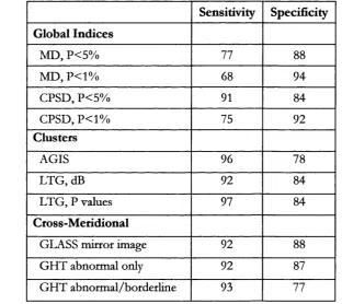
1.5.6 Comparison o f detection systems...61
1.6 Detecting Glaucomatous Visual Field Progression... 64
1.6.1 Observer O pinion... 64
1.6.2 Global Indices...64
1.6.3 Cluster Analysis...65
1.6.4 Statpac I I Glaucoma Change Probability Analysis... 66
1.6.5 Linear regression...68
1.6.5.1 Use o f linear regression in field progression... 71
1.6.6 Neural Networks... 78
1.6.7 Field conversion in O H T ...80
1.6.8 Non-Glaucomatous Visual Field Change... 80
1.7 Interventions in Glaucoma...81
1.8 Justification and A im s...83
2 M ethod...85
2.1 MRC 5-FU Treatment T ria l...85
2.1.1 Inclusion Criteria... 85
2.1.2 Exclusion Criteria... 86
2.2 Clinical Examination/Tests...89
2.2.1 Refraction... 89
2.2.2 Visual A cuity... 90
2.2.2.1 Distance visual acuity assessment... 90
2.2.2.2 Near Visual acuity assessment...91
2.2.3 Intraocular Pressure...91
2.2.4 Grading o f Lens O pacity...92
2.3 Visual Field Testing... 93
2.3.1 Preoperative Visual Field Testing... 94
2.3.2 Postoperative Visual Field Testing... 94
2.3.3 Refractive Correction for visual field testing... 94
2.3.4 Pupil Size and field testing... 94
2.4 Analysis o f Visual Field Data... 95
2.4.1 Statpac Global Field Indices... 95
2.4.2 Statpac I I Glaucoma Change Probability Analysis...96
2.4.3 AGIS grading...96
2.4.4 Pointwise Linear Regression Analysis (PLR)... 97
2.4.5.1 Basic analysis...99
2.4.5.2 Slope analysis... 99
2.4.5.3 Spatial Change C riteria... 99
2.4.5.4 Temporal Change C riterion... 102
2.4.5.5 Excessive Point V ariability... 102
2.4.5.6 Comparison o f Change Across the Horizontal Midhne... 102
2.4.5.V Random Analysis...103
2.4.5.8 Mean Slope and Threshold o f Changing Points...103
2.4.6 Comparison o f Progressors and Non-progressors... 103
2.5 Validation o f PLR progression criteria... 104
3 Results...105
3.1 FoUow-up o f patients w ithin tria l... 105
3.1.1 lO P changes following trabeculectomy... 106
3.1.2 Visual Acuity and Foveal Threshold Following Trabeculectomy... 106
3.1.3 Cataract Grading...107
3.2 Statpac Analysis... 110
3.2.1 Changes in STATPAC global indices... 110
3.2.2 Linear regression analysis o f global indices...I l l 3.2.3 Pointwise analysis using Glaucoma Change Probabihty analysis... I l l 3.2.4 AGIS scoring...112
3.2.5 Correlation o f global indices w ith lO P ... 112
3.3 Pointwise linear regression... 113
3.3.1 Basic Analysis...113
3.3.2 Slope Analysis... 115
3.3.3 Spatial Change C riteria...117
3.3.4 Temporal Change C riterion... 122
3.3.6 Comparison o f Change Across the Horizontal M idline...126
3.3.7 Random Analysis... 129
3.3.8 Mean Slope and Baseline Threshold o f Changing Points...131
3.4 Progression criteria and change...132
3.5 Progression criteria and media opacity...133
3.6 Progression criteria and Median lO P ... 136
3.6.1 Extended follow up o f original 56 patients from 6 to 8 fields... 141
3.6.2 Application o f learning set criteria to test patients...143
4 Discussion... 147
4.1 Intraocular pressure reduction follow ing trabeculectomy...147
4.2 Changes in media opacity and visual acuity following trabeculectomy...148
4.3 Statpac analysis... 151
4.3.1 Global indices o f visual field change... 151
4.3.2 Pointwise analysis using Glaucoma Change Probability analysis...152
4.3.3 AGIS scoring...152
4.4 PLR progression criteria... 153
4.5 Application o f criteria to additional data... 157
4.5.1 Extended follow up o f original 56 patients from 6 to 8 fields... 157
4.5.2 Application o f learning set criteria to test patients... 158
4.5.3 Optimal progression criteria... 158
5 Conclusion... 165
6 References... 166
List o f figures
Figure 1 Humphrey Field Analyzer M k I I ... 31
Figure 2 Octopus 101 and 1-2-3 perimeters...32
Figure 3 Dicon LD400 perimeter...32
Figure 4 Full threshold staircase strategy as used the Humphrey Field Analyzer... 33
Figure 5 Intraindividual intertest variation — in dB...40
Figure 6 Loss o f sensitivity in dB per decade across the central 30°... 44
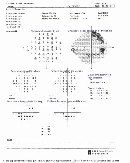
Figure 7 The Statpac printout from the Humphrey Field Analyzer... 53
Figure 8 Cluster arrangement for the AGIS scoring system... 54
Figure 9 Statpac Glaucoma Change Probability Printout...67
Figure 10 Regression line fitted to data set so as to rninimize the squares o f the residuals 69 Figure 11 Spatial filtering o f a visual fie ld ... 79
Figure 12 Lens Opacities Classification System I I I ...93
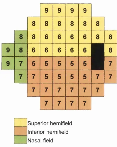
Figure 13 Clusters in the Glaucoma Hemifield Test and Perimetric Nerve Fibre Bundle Map... 100
Figure 14 Mean lO P in the MRC 5-FU following trabeculectomy...106
Figure 15 Modified LOGS grading at baseline and 12 months... 108
Figure 16 Near and Distance LogMar V A Versus Foveal Threshold at 16 Months 109 Figure 17 Distribution o f change in M D , PSD, logMAR distance V A and foveal threshold at 16 months... 110
Figure 18 Whole field Glaucoma Change Probability analysis at 16 months...112
Figure 19 Numbers o f e yes showing change against P value. 6 fields... 114
Figure 20 No. o f eyes showing change v slope. 6 fields, 1-5 points, P< 0.05... 116
Figure 22 Change criterion - 3 contiguous points, 6 fields. Slope = 1 dB /yr. Number o f
eyes showing change against P value...118
Figure 23 Change criterion - 2 points in a G H T cluster, Slope=l dB /yr, 6 fields. Numbers
o f eyes showing change against P value... 119
Figure 24 Change criterion - any 2 points in a perimetric nerve fibre bundle, 6 fields. Slope
= 1 dB /yr. Numbers o f eyes showing change against P value...120
Figure 25 Change criterion - any 2 points in area covered by G H T, 6 fields. Slope = 1
dB /yr. Numbers o f eyes showing change against P value... 120
Figure 26 Change criterion — 1-5 points, 6 Filtered Fields. Slope=l dB /yr. Numbers o f
eyes showing change against P value...121
Figure 27 Numbers o f eyes showing change at same point at 5 and 6 fields. 1, 2, or 3
points, Slope=l d B /yr... 123
Figure 28 Change criterion — 6 fields, blind spot points removed, 1 -5 points,
S lope=ldB /yr. Change against varying P value... 124
Figure 29 Number o f eyes showing change when the Critical Slope is doubled for
peripheral points. 1 or 4 points. 6 fields. Critical slope centrally = 1 d B /yr... 125
Figure 30 Number o f eyes showing change when the P value is halved fo r peripheral
points. 1 or 4 points. 6 fields, P value centrally <0.05... 126
Figure 31 Change criterion - Difference o f 1, 2, or 3 changing points between vertical
hemifields. 6 fields. Slope =1 dB /yr. Change versus P value...127
Figure 32 Change criterion - Difference between 2 symmetrical G H T clusters o f at least 2
significant points, 6 fields, Slope=l d B /yr...129
Figure 33 Number o f eyes showing change against P value, 6 randomised fields. Slope =1
d B /yr... 130
Figure 34 Mean slope o f changing points versus P value. N o minimum critical slope is
Figure 35 Mean slope o f significantiy changing points in randomised field series. No
minimum critical slope is required... 131
Figure 36 Mean baseline sensitivity o f points changing over 6 fields. N o minimal slope is required... 132
Figure 37 Mean baseline sensitivity o f points changing over 6 randomised fields. No minimal slope is required... 132
Figure 38 Change shown in individual trial patients using PLR, Statpac II, and AGIS progression criteria over 6 fields... 134
Figure 39 Box-whisker plot explanation... 136
Figure 40 Median change in foveal threshold for the 6 exclusive progression criteria over 6 fields...137
Figure 41 Median change in logMAR V A for the 6 exclusive progression criteria over 6 fields...138
Figure 42 Median lO P for progressors and non-progressors... 139
Figure 43 Median % fall in lO P for progressors and non-progressors... 140
Figure 44 Extended follow up - 5 points changing vs slope, P<0.05... 141
Figure 45 Extended follow up - 3 contiguous points...141
Figure 46 Extended follow up - 2 points in a Glaucoma Hemifield Test cluster...142
Figure 47 Extended follow up - 2 points in a Perimetric Nerve Fibre Bundle Cluster...142
Figure 48 Extended follow up - 4 point difference between vertical hem ifields...142
Figure 49 Extended follow up - 3 points changing over 5 & 6 or 7 & 8 fields...143
Figure 50 Learning/ test sets - 5 points changing vs. slope, P<0.05... 144
Figure 51 Learning/ test sets - 3 contiguous points... 144
Figure 52 Learning/ test sets - 2 points in a Glaucoma Hemifield Test cluster...145
Figure 53 Learning/ test sets - 2 points in a Perimetric Nerve Fibre Bundle Cluster 145 Figure 54 Learning/ test sets - 4 point difference between vertical hem ifield... 146
List of tables
Table 1 Distribution o f field test techniques according to the RCOphth Trabeculectomy
A udit... 29
Table 2 CIGTS scoring system... 52
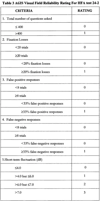
Table 3 AGIS Visual Field Reliability Rating For HFA test 24-2... 56
Table 4 Sensitivity and specificity o f single and repeat visual field testing using the G H T to classify visual field test results... 59
Table 5 Sensitivity and specificity o f 10 algorithms for detecting glaucomatous field loss. 63 Table 6 Change Criteria Used in Studies o f Pointwise Linear Regression...76
Table 7 Tests performed on each visit o f the MRC 5-FU trial... 88
Table 8 MRC 5-FU trial recruitment and patient progress as o f 2 8 /2 /9 8 ... 105
Table 9 Baseline characteristics o f the 56 trial patients in the initial analysis... 106
Table 10 Mean visual acuity and foveal threshold at baseline, 12 and 16 months... 107
Table 11 Correlation Between Foveal Threshold and Best Corrected logMAR Visual Acuity ... 109
Table 12 Statpac Global Indices for each post operative visit from baseline — 16 months. ... I l l Table 13 Pearson correlation between change in lO P and change in global Statpac values at 16 months...113
Table 14 Baseline characteristics o f the 97 test patients that formed the test group 143 Table 15 Numbers o f patients requiring cataract surgery in the AGIS study...150
Table 16 Percentage o f exclusive progression detected using 2 criteria, and 3 data sets... 159
Table 17 Power calculation from the MRC 5-FU Filtration Surgery Study... 162
List of abbreviations
5FU 5-fluorouracil
asb apostilb
AGIS Advanced Glaucoma Intervention Study
A L T argon laser trabeculoplasty
C cortical
C-D cup-disc
CIGTS Collaborative Initial Glaucoma Treatment Study
CNTG Collaborative Normal Tension Glaucoma
CPSD corrected pattern standard deviation
DCCT Diabetics Control and Complications Trial
dB decibel
EM G T Early Manifest Glaucoma Trial
ETDRS Early Treatment o f Diabetic Retinopathy Study
FovTh foveal threshold
G H general height
G H T glaucoma hemifield test
GLASS Glaucoma Screening Study
HFA Humphrey field analyzer
lO L intraocular lens
lO P intraocular pressure
LE D light em itting diode
LOCS lens opacity classification system
logMAR loganthm o f minimum angle o f resolution
LONS LongitTudinal Optic Neuritis Study
M D mean deviation
M EH Moorfields Eye Hospital
MMC mitomycin c
mtnHg millimetres o f mercury
MPS Macular Photocoagulation Study
MRC medical research council
N FL nerve fibre layer
NC nuclear colour
N O nuclear opalescence
N IH National Institutes o f Health
N TG normal tension glaucoma
O N TT Optic Neuritis Treatment Trial
O H T ocular hypertension
PERK Prospective Evaluation o f Radial Keratotomy
PLR pointwise linear regression
PNFB perimetric nerve fibre bundle cluster
POAG primary open angle glaucoma
PSCLO posterior subcapsular lens opacity
PSD pattern standard deviation
RAFEP regression analysis w ith fixed effects on panel data
RCOphth Royal College o f Ophthalmology
SF short-term fluctuation
Sig
significanceSITA Swedish interactive threshold algorithm
SLO scanning laser ophthalmoscope
UCL University College London
Acknowledgements
I would like to thank the following for their help in producing this thesis;
Peng T Khaw for selecting me to work on the 5-FU trial and supervising this thesis.
Fred Fitzke also supervised this thesis and gave up time fo r numerous meetings about
progression criteria.
Roger Hitchings provided support and constructive criticism.
Aachel Kotecha, Tom Lowe and Rachel Michell worked w ith me on the 5-FU trial, the
data collected reflects their efforts as much as mine.
David Crabb for general support plus allowing me to use figure 11
Andromachi Frangouh who helped provide additional field data.
The MRC 5-FU trial is funded by the Medical research Council o f Great Britain, grant
Statement of originality
The work presented in this thesis was undertaken by myself at the Institute o f
Ophthalmology, London and at Moorfields Eye Hospital, London. The data was collected
from an ongoing clinical trial based at Moorfields. My co-workers on the trial are
acknowledged above. The thesis and data analysis represent my own work helped by the
1
Introduction
L I Ocular Changes in Glaucoma
Glaucoma is a progressive optic neuropathy w ith characteristic structural damage to
the optic nerve and characteristic visual field defects (Gupta and Weinreb 1997). A recent
estimate put the number o f people bilaterally blind from glaucoma by the year 2000 at 6.7
m illion (Quigley 1996). It is generally assumed that the glaucomatous disease process is
modifiable by treatment. Attempts have therefore been made to reduce the impact o f
glaucoma by improved detection o f cases and improved treatment. Hindering such efforts
is the fact that no single measurable variable (such as blood pressure, or blood sugar) exists
for diagnosing glaucoma and that there remains no ideal single method for following a
patient once the condition has been diagnosed. Three broad areas are examined in clinical
settings: intraocular pressure; optic disc and nerve fibre layer; and visual fields.
Although an abnormality in one area may be strongly indicative o f glaucoma, it
usually requires an abnormality in more than one area for a diagnosis to be made. The
detection and monitoring o f glaucoma w ith respect to these three areas is discussed in the
next 3 sections.
1.1.1 Intraocular Pressure
Intraocular pressure (lOP) is no longer included in the definition o f glaucoma.
However it has been linked to it from the earliest description o f the condition, where a
hard painful eye was linked to blindness. Recently our views on the relationship between
intraocular pressure and glaucoma have changed. Many epidemiological surveys have
quantified the distribution o f lO P in various populations and have established that the
mean lO P is around 15-16 mmHg (Armaly 1965; Bankes et al. 1968; Kahn et al. 1977;
Sommer et al. 1991; Klein et al. 1992; Bonomi et al. 1997). The mean can vary for different
tonometer) (Arkell et a l 1987) and Mongolians (12,7 mmHg in men tested using a
Goldmann tonometer) (Foster et al. 1996) than Caucasians (Armaly 1965; Bankes et al,
1968; Kahn et al, 1977; Sommer et al, 1991; Klein et al, 1992; Bonom i et al, 1997),
Furthermore the distribution is not normal. Despite this lO P has frequently been analysed
as though it were so (Colton and Ederer 1980), In particular the concept has developed
that the upper normal Hmit o f intraocular pressure is the mean + 2 standard deviations or
approximately 21 mmHg, Given the fact that the distribution is not normal, it is not
reasonable to use the figure o f 21 as the cut o ff between normal
(^1
mmHg) andabnormal (>21 mmHg) in such a way.
Even though one cannot say that an lO P above a certain point is abnormal, raised
intraocular pressure undoubtedly does play a significant role in the pathogenesis o f
glaucomatous damage. Unilateral conditions that produce raised lO P frequently lead to
unilateral field loss. Several groups have retrospectively studied the association between
intraocular pressure and visual field loss finding that increased intraocular pressure leads to
an increased likelihood o f visual field loss (Sommer 1989) and an accelerated rate o f loss
(Jay and Murdoch 1993), Other work has shown an association between optic disc changes
and lO P in normal (Jonas et al, 1998) and high-tension glaucoma (Varma et al, 1995), A
non systematic review by Palmberg showed an association between lO P and progression in
glaucoma treatment studies (Palmberg 1996), Prospective epidemiological studies have
shown an increasing risk o f glaucoma w ith raised intraocular pressure (Armaly et al, 1980;
Sommer et al, 1991; Dielemans et al, 1994; Leske et al, 1995; Leske et al, 2001), However
at the same time the same studies have pointed out that 40-55% o f their subjects w ith
glaucoma had lO P ’s below 21 mmHg at screening (Sommer et al. 1991; Dielemans et al,
1994; Leske et al, 2001), The influence o f factors other than lO P is shown in data from
the Baltimore Eye Study (Sommer et al, 1991), The prevalence o f glaucoma among black
subjects was 4,3 times that o f white subjects yet there was no difference in the mean lO P ’s
Despite a large number o f treatment studies very little hard evidence exists to show
that, in patients w ith glaucoma, lowering lO P reduces the rate o f visual field progression.
Two retrospective studies have shown some benefit from lowering lO P (Mao et al. 1991;
Odberg 1993). In a systematic review o f trials o f glaucoma treatment Rossetti showed that
glaucoma treatment is associated w ith a reduction in intraocular pressure (Rossetti et al.
1993). A t the time that the paper was w ritten only 3 randomised controlled trials w ith data
on visual fields were available (Epstein et al. 1989; Kass et al. 1989; Schulzer et al. 1991).
Their statistical combination failed to show a significant protective effect o f active
treatment. A subsequent prospective study randomising glaucoma patients to drops, argon
laser trabeculoplasty (ALT) or trabeculectomy found that the differences in TOP between
the A L T and trabeculectomy patients explained the differences in field progression
between the 2 groups (Migdal et al. 1994). Despite similar mean TOP values in the laser
and medical groups the greater deterioration o f visual fields in the medical group allowed
the authors to conclude that “ medical treatment appears to make the fields worse, or allows
them to deteriorate faster, in some way beyond its effect on the lO P ” . The Glaucoma
Laser T rial randomised both eyes o f patients w ith glaucoma to initially receive argon laser
trabeculoplasty in one eye and tdmoptol 0.5% in the other (Glaucoma Laser Trial Research
Group 1991). Additional treatment was prescribed according to a pre-defined list o f
additional topical treatments. Eyes initially receiving A L T had a consistently lower lO P
than those initially receiving tim optol. Automated field test results firom the initial study
when the bulk o f the patients were still under follow up showed a trend for improvement
in the fields in both arms o f the trial. It was only w ith extended follow up after 4 years that
quantitative and qualitative grading o f fields showed more fields deteriorating than
im proving in either arm. Unfortunately at 4 years the follow-up rate was only 120/271
patients (Glaucoma Laser Trial Research Group 1995). A t this point the mean point
sensitivity in the A L T group was 0.7 dB higher than at enrolment, whereas the figure in the
was more negative, boJh arms had a majority o f patients w ith deteriorating discs. There
was no significant difference in the changes between the two arms. The researchers were
thus only able to claim that initial treatment w ith A LT was at least as efficacious as initial
treatment w ith topical medication. Despite the lower TOP achieved using A L T they were
unable to make any claims linking lO P and automated visual field changes. In the
Advanced Glaucoma Intervention Study the patients were randomised to different
sequences o f treatment using A L T and trabeculectomy (AGIS 1994). Claiming
“ unexpected findings of statistically significant interactions” the authors published their
results separately for black and white patients (AGIS 1998). Having done this they felt that
better visual field preservation only occurred in white patients who achieved better lO P
reduction. The lack o f concordance between lO P lowering and field preservation in black
patients was they felt due to other factors. The only discussion o f potential factors is a
reference to a review that cites age, race, myopia, and vascular haemodynamics as having a
role in the development and progression o f glaucomatous visual fields (Drance 1997).
Airaksinen followed the optic discs from normal, ocular hypertensive and glaucoma
subjects for 5 years using planimetry to quantify any changes (Airaksinen et al. 1992).
None o f the normals showed any change in tim area while 79% o f the glaucoma subjects
and 43% o f the ocular hypertensives did. Further analysis showed that 90% o f the change
in rim area loss over time was accounted for by variables other than the ones measured in
the study namely age, disc area, initial rim area and lOP. There was a weak correlation
between rate o f rim area change and lO P (R^ = 0.058, P<0.05) that was weaker than that
seen w ith age (R^ = 0.09, P<0.01).
There is little evidence linking the role o f lO P in the conversion o f eyes w ith ocular
hypertension to glaucoma. Prospective (Kitazawa et al. 1977) and retrospective (David et
al. 1977; Odberg 1993) studies o f patients w ith ocular hypertension have failed to find an
association between lO P and those patients who develop field loss. In a prospective study
greater rate o f field conversion than the tim optol group (Kass et al. 1989). The mean TOP
in the tim optol group was lower than in the placebo group. No statistical comparison o f
t o p’s for all patients converting versus those who did not was given. Finally in a
retrospective study o f irabeculectomy patients TOP could not predict which patients would
show deterioration o f visual field (TCidd and M 1985).
The Collaborative Normal-Tension Glaucoma Study Group randomised patients
w ith normal tension glaucoma to no treatment or to treatment designed to lower their TOP
by 30% (Collaborative Normal-Tension Glaucoma Study Group 1998; Collaborative
Normal-Tension Glaucoma Study Group 1998). The treated arm experienced less visual
field progression. However the only link between TOP and field progression was obtained
when data regarding patients developing cataract was censored.
The lack o f conclusive evidence between TOP and glaucoma progression has led to
the establishment o f the Early Manifest Glaucoma Trial (EMGT) to evaluate the
effectiveness o f reducing TOP in early, previously untreated open-angle glaucoma. Patients
w ith to p’s <30 mmHg and w ith m ild field loss have been randomised to either treatment
or no treatment at all. Both arms wiU be closely monitored (Leske et al. 1999).
Intraocular pressure remains a risk factor but is not the sole mechanism by which
glaucomatous damage occurs. Measuring TOP has some value in detecting patients w ith
high pressures who are at increased risk o f developing glaucoma. Similarly measuring TOP
has some role in m onitoring patients undergoing treatment. Other than at extremely high
levels TOP cannot be excTusively rehed upon to diagnose or m onitor glaucoma.
1.1.2 Optic D isc
The normal and glaucomatous nerve fibre layer and optic disc have been studied
w ith a view to developing strategies to detect and m onitor glaucomatous damage. Both
Crucial to using the optic disc to detect glaucoma is the ability to decide what
constitutes a normal disc. The size and variability o f normal and glaucomatous discs in
black and white populations has been defined using a population based study (Varma et al.
1994). Normal discs are variable in size w ith significant racial and sexual variations. In
blacks the optic disc is approximately 12% larger than in whites. Blacks also show a larger
interindividual variation in their disc area varying from 0.9 to 6.28mm^ while whites vary
from 1.15 to 4.94 mm^ (Varma et al. 1994). Male optic discs are on average 2-3% larger
than female optic discs (Varma et al. 1994).
Further study o f disc components reveals further variability. The neuroretinal rim
area is proportional to disc size in blacks and whites (Britton et al. 1987; CaprioU and M iller
1987; Varma et al. 1994). However the lim its o f normality for rim area cover a very large
range from 0.7 mm^ to more than 4 mm^. The regression slope o f rim area against disc
area is smaller for blacks than whites (Varma et al. 1994) suggesting that as black optic discs
increase in size there is a smaller increase in rim area compared to white optic discs. For
any given disc size the rim area is lower in blacks than in whites (Varma et al. 1994). It has
also been shown that larger optic discs have a greater number o f nerve fibres in humans
(Jonas et al. 1992) and monkeys (Quigley et al. 1991). Since rim area increases w ith disc
size it is likely that rim area is an indirect marker for the number o f nerve fibres in an optic
disc. Thus it has been suggested that for any given disc size a black optic disc w ill contain
fewer nerve fibres than a white one (Varma et al. 1994). In glaucoma it is the death o f
ganglion cells that produces visual loss (Wygnanski et al. 1995). In itia l reports o f
photoreceptor death (Panda and Jonas 1992) in glaucoma have not been confirmed in
subsequent reports (Kendell et al. 1995; Wygnanski et al. 1995). The earliest visible
changes due to ganglion cell death in glaucoma are defects in the retinal nerve fibre layer
(Hoyt and Newman 1972). The changes may be seen as a diffuse thinning or as wedge
shaped defects in the retinal nerve fibre layer. These changes may precede optic disc and
themselves be preceded by an optic disc haemorrhage (Airaksinen et al. 1981). W ith
progressive fibre loss the N FL becomes thinner and/or wedge shaped defects enlarge.
When sufficient ganglion cells are lost, optic disc morphology changes. The
changes seen can be variable. Diffuse neural rim thinning, vertical elongation o f the cup,
rim notch formation, or pallor o f the rim w ith no change in outline have aU been described
(Airaksinen et al. 1992). The loss o f ganglion cells also leads to alterations in the position
o f blood vessels, the loss o f rim tissue removes support for the vessels. Changes in the
optic disc may precede development o f visual field defects (Sommer et al. 1979; M otolko
and Drance 1981; Funk 1991; Zeyen and CaprioH 1993; Kamal et al. 1999).
W ith progressive ganglion cell death there is an increase in cup size and in the cup-
disc (C-D) ratio. Cup size and C-D ratio are both a function o f the size o f the optic disc
and rim area, which as mentioned above, vary quite considerably in the normal population.
Inter observer agreement in detecting C-D ratio is poor (Lichter 1976; Varma et al. 1989;
Varma et al. 1992).
Another feature o f human glaucomatous eyes is an outward bowing o f the lamina
cribrosa (Quigley et al. 1983). This has also been observed in an animal model o f glaucoma
(Coleman et al. 1991). It is believed that bowing can cause kinking o f axons, interrupt
axonal transport and thus cause cell death. Reduced connective tissue support in the
superior and inferior quadrants o f the optic disc is believed to contribute to the preferential
loss o f axons at these sites (Quigley and Addicks 1981; M iller and Quigley 1988). Such
preferential loss produces vertical enlargement o f the optic cup. Where the rate o f loss o f
ganglion cells is asymmetric between the eyes the optic cup size w ill also be asymmetric.
The accelerated loss o f ganglion cells in glaucoma leads to a reduction in rim area
that is greater than the natural decline seen w ith age (Airaksinen et al. 1992). However it
has not beem possible to discriminate between normal and glaucomatous eyes using rim
area because o f the overlap between the two groups (Caprioli 1992; Damms and Dannheim
Several studies have looked at the sensitivity and specificity o f techniques for
separating glaucomatous from normal optic discs. Features assessed include vertical C-D
ratio (Damms and Dannheim 1993), photographs o f nerve fibre layer defects (Airaksinen
et al. 1984), circumhnear vessel baring (Balazsi and Wemer 1983), and scanning laser
ophthalmoscope (SLO) images (WoUstein et al. 1998). When assessing the impact o f these
studies it is important to look at the patient selection. Using features in disc photographs
from a screened population in the Baltimore Eye Study shows that there is no cu t-o ff point
for vertical C-D ratio or narrowest rim w idth when separating normal optic disc from
glaucomatous ones (Tielsch et al. 1991). Using quantitative techniques, such as planimetry
and digitised image analysis o f videographic images, to predict field loss from optic disc
features the best sensitivity obtainable was 74% (O' Connor et al. 1993). This figure was
achieved by obtaining nerve fibre height measurements; poor specificity reduced the
diagnostic precision value to 68%. (Diagnostic precision = the total proportion o f eyes that
were correctly identified as having healthy or glaucomatous eyes). The same article found
that qualitative assessments based on optic disc and nerve fibre photographs had higher
levels o f diagnostic precision. By analysing SLO images, high sensitivity and specificity at
separating glaucomatous disc from normal ones have been obtained. Using the 99%
prediction interval from the linear regression between the optic disc area and the log o f the
neuroretinal rim area 96.3% specificity and 84.3% sensitivity were produced (WoUstein et
al. 1998). W ith this technique we may be closer to an objective technique for separating
early glaucomatous eyes from normal ones. However this analysis technique has not been
tested on its ability to m onitor disease progression, nor has it yet been used in a large
population study, being derived from a hospital population.
Serial examinations o f the optic disc and nerve fibre layer have tried to establish the
temporal link between optic disc and visual field changes. In a study o f 813 ocular
hypertensive eyes examined annuaUy over 5 years Quigley et al were able to identify 37 eyes
The authors compared optic disc and nerve fibre layer photographs in the 2 subgroups.
Disc change was detected in only 19% o f converters, while progressive nerve fibre layer
atrophy was observed in 49% o f converters. A smaller study followed one eye from 15
patients over 6 years (Zeyen and Caprioli 1993). Eight eyes w ith an initially normal visual
field showed disc changes using planimetry; six o f these eyes did not develop field
abnormalities. Population studies have also highlighted the mismatch between optic disc
and visual field changes. In the Beaver Dam Eye Study o f the 104 cases o f “ definite”
POAG 45 had high TOP, abnormal visual fields, but normal stereo disc photographs (Klein
et al. 1992).
Segmental analysis o f the optic disc using either planimetry (Weber et al. 1990) or
more frequently the scanning laser ophthalmoscope (Asawaphureekom et al. 1996; Anton
et al. 1997; Yamagishi et al. 1997; Anton et al. 1998)has shown a correlation between focal
disc changes and regional visual field loss. However problems remain w ith considerable
interindividual variability in optic nerve head size and configuration; some field zones
topographically map to certain optic disc rim areas w ith greater predictability than others
(Yamagishi et al. 1997; Anton et al. 1998).
1.1.3 Visual Field
The visual field o f an eye refers to all the space that can be seen at any given
instant. The visual field is quantified by presenting hght stim uli and determining whether
the eye can see them or not. It requires that not only is an image formed w ithin the eye but
inform ation about the image must be transmitted to the brain and then “ perceived” . The
stim uli used to map a visual field may be static or moving, and can have variable size and
intensity. The stim uli may be projected on to a flat surface so that more peripheral stim uli
are further from the eye (Campimetry), or they may be projected onto a curved surface or
bowl, thus keeping the stimulus-eye distance constant. A n isoptre is an imaginary Hne
between isoptres is known then a 3 dimensional model o f sensitivity can be constructed.
Although not the first person to map the visual field it was Traquair who coined the phrase
“ h ill, or island, o f vision” to describe the decrease in sensitivity to hght as one moves
peripherally.
It has been suggested that early glaucoma produces a generahsed contraction o f
isoptres/ reduction in sensitivity (Anctil and Anderson 1984; Caprioh et al. 1987; Drance
1991). Other work has tended to contradict this view suggesting that early signs o f
glaucoma in the visual field are represented by regional depressions in sensitivity or
scotomas (Wemer and Drance 1977). Indeed specific attempts to detect fields w ith diffuse
loss purely due to glaucoma have been unsuccessful (Wemer et al. 1982; H eijl 1989; Asman
and H eijl 1994). Asman and H eijl using the glaucoma hemifield test found that only 2 out
o f 1582 eyes showed diffuse field loss (Asman and H eijl 1994). Some o f the discrepancies
between papers over their detection o f diffuse loss have been attributable to methodology:
static vs. kinetic perimetry, the confounding effect o f miosis and cataract, patient selection
and the technique used to detect depression. Global indices (Caprioh et al. 1987) have
been used to indicate diffuse depression rather than specific algorithms (Asman and H eijl
1994). Recent work that took into account the presence o f lens opacity saw the incidence
o f diffuse loss in early glaucoma faU from 12.4% to 4.4% once patients w ith cataract were
excluded (Chauhan et al. 1997). Henson, using patients w ith estabhshed early field loss, has
argued that diffuse loss is present as a component o f the total field loss (Henson et al.
1999). The results o f his study differ from those o f H eijl’s (H eijl 1989) even though both
use the same technique measuring the sensitivity o f the 10 best points in the field.
However H eijl’s conclusions were based on eyes that may weU have had even earlier field
loss, indeed 2 o f them had no field loss at all.
It is now recognised that isolated defects represent the more common initial field
defect in glaucoma (Drance 1969). The position o f these can be paracentral, nasal or
scotoma the visual field displays an increase in short term fluctuation (Flammer et al. 1984)
in the threshold sensitivity to hght.
Progression o f glaucoma is manifest by 1) scotomas becoming deeper 2)
enlargement o f scotomas and 3) development o f new scotomas (Mikelberg and Drance
1984). Despite our knowledge o f glaucomatous field progression the ability o f bumans to
agree on which field series are progressing is poor (Wemer et al. 1988). Furthermore
algorithms to select deteriorating fields from stable ones are also not good enough for the
algorithm to be rehed upon alone (Smith et al. 1996).
The loss o f visual field represents a late sign o f damage in glaucoma. In post
mortem studies Quigley has shown that 25-50% o f neurons die before detection o f field
loss using manual perimetry. W ith automated perimetry a loss o f 20% o f ganghon cells
correlates w ith approximately a 5dB loss o f sensitivity and a 40% loss o f ganghon cells
correlates w ith approximately a 10 dB reduction. These studies by their very nature are
retrospective and small in size making comparisons difficult. The automated perimetry
study consists o f only 6 eyes, ah taken from patients age 70 or older (Quigley et al. 1989).
The manual perimetry study consists o f 26 eyes, w ith donors being as young as 46 (Quigley
et al. 1982).
Early perimetry concentrated on using white sfimuh on white backgrounds. In an
attempt to detect visual loss earher in the glaucomatous disease process, other testing
modahties have been tried. In glaucoma there is inifiahy a greater loss o f large ganghon
ceUs. The loss occurs in humans (Quigley et al. 1987; Quigley et al. 1988) and in monkeys
(Glovinsky et al. 1991; Glovinsky et al. 1993; Wygnanski et al. 1995; Desatmk et al. 1996)
and occurs centraUy as weh as peripheraUy (Wygnanski et al. 1995). The preferential loss o f
larger neurons has stimulated interest because it is known from rhesus monkey studies that
the optic nerve contains principaUy 2 types o f neuron. Ninety percent are the smaher
diameter slower conducting P cehs, the remaining 10% percent are mainly the larger
contrast gain, and are believed to be involved in motion detection and to preferentially
receive inpxrts from cones sensitive to shorter wavelengths. The preferential loss o f M cells
in glaucoma has led to field testing using short-wave perimetry (Johnson et al. 1993;
Johnson et al. 1993), motion detection (Fitzke et al. 1989), contrast sensitivity (Arden and
Jacobson 1978), and flicker (Lachenmayr et al. 1991; Lachenmayr et al. 1991; Yoshiyama
and Johnson 1997). Recent work has challenged the idea that test modalities that are
selective for a particular type o f cell death w ill offer any benefits in the detection o f
glaucoma (Johnson et al. 2000). Shrinkage in ganglion cell size prior to death may be
causing an artefactual loss in large ganghon cells. A t present white on white perimetry
remains the dominant field testing technique in the United Kingdom. Table 1 shows the
type o f field test used on patients included in the Royal College o f Ophthalmologists
trabeculectomy audit (Beth Edmunds — personal communication).
A major problem w ith visual field testing are the intertest fluctuations at individual
points that make detection o f change over successive fields d ifficu lt (H eijl et al. 1987; H eijl
et al. 1989). Fluctuation between field tests can lead to a false impression o f change, w ith
fields appearing to improve as well as progress. As wiU be discussed later a variety o f data
acquisition and analysis techniques have been developed to improve the detection o f
glaucoma and to improvement the m onitoring o f the disease.
N o technique has yet been shown to have overall superiority in detecting and
m onitoring glaucoma. In the future, sophisticated optic disc analysis may offer this. A t the
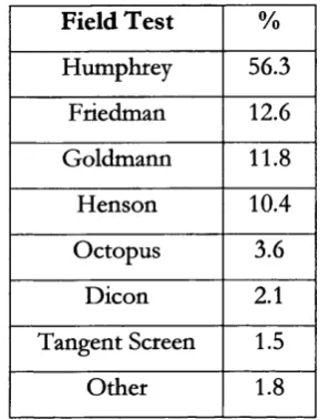
Table 1 Distribution of field test techniques according to the RCOphth Trabeculectomy Audit.
Field Test %
Humphrey 56.3
Friedman 12.6
Goldmann 11.8
Henson 10.4
Octopus 3.6
Dicon 2.1
Tangent Screen 1.5
Other 1.8
Automated perimetry (Humphrey, Henson, Octopus and Dicon) is used on over 70% of the patients in the audit; while kinetic perimetry (Goldmann and tangent screen) is used to test less than 15%.
1.2 A u to m ated p e rim e try fo r m easu rin g visu al fie ld s
The first formal attempts at measuring the visual field were performed by Young in
1801. F ifty years later in 1856 von Graefe published his accounts o f campimetry, the
plotting o f visual fields on a flat surface. He mapped the blind spot, scotomas,
hemianopsias, and described isopter contraction. The following decade Forster, using an
Arc perimeter, extended the area tested to beyond 45 degrees. In the 1950’s Goldmann
developed his hemispheric projection perimeter that is still in use today. He also quantified
the relationship between the area and luminance o f a test object.
Early visual field work was based around the concept o f kinetic perimetry; the
subject indicates when a moving stimulus can first be seen. In 1939 Sloan described the
use o f static perimetry wherein the stimulus is not moved but its intensity is varied. Harms
and Aulhom went on to design the Tübinger perimeter that permitted static and kinetic
perimetry. Subsequently the Armaly screen was developed. It uses a combination o f
kinetic and static manual perimetry on a Goldmann perimeter to screen a patient for
glaucomatous field defects. A t most points stim uli o f variable size and intensity are
are mapped using standard kinetic techniques (Rock et al, 1971; Rock et al. 1973). This
technique produced fast test times w ith high sensitivity and specificity figures fo r separating
patients with glaucomatous field loss from normals. The test is not widely used but the
point locations used have been incorporated into screening programs available in the
Humphrey field analyser. Although attempted by others in the early 1960’s, Lynn and Tate
were the first to demonstrate an automated static perimeter in 1969. The rapid change in
technology over the next 30 years has led to the development o f modem automated
perimeters the most popular o f which is the Humphrey Field Analyzer (table 1).
1.2.1 Humphrey Field Analyzer
The Humphrey Field Analyzer (AUergan-Humphrey, San Leandro, Cahfomia,
USA) is a projection automatic perimeter. Models I and I I consist o f a single unit
containing a projection bowl, a display screen for entering inform ation, a printer and data
storage facilities in the form o f a floppy disk (I and II) or hard drive (II). Visual field
testing is performed w ith the patient facing the stimulus bowl, a white hemispherical bowl
w ith a radius o f 330 mm. Two diffuse hght sources are used to illuminate the bowl so that
the background luminance is 31.5 asb. The illum ination is checked when the machine is
switched on and at the beginning o f each test w ith the patient seated in front o f the bowl.
In addition the local background luminance is tested before each stimulus is presented so
that stimulus intensity may be adjusted to cope w ith any local variations in background
luminance. Spot stimuh lasting 0.2s are projected on to the surface o f the bowl using a
m irror. Step motors control the position o f the m irror. Using neutral density filters,
stimulus strength can be varied from 0.08 to 10,000 asb (51 dB). Stimulus size can be
varied to match the 5 sizes (V to I) available on the Goldman perimeter. Coloured filters
Figure 1 Humphrey Field Analyzer Mk II
n
1
The Humphrey offers screening and threshold strategies (see below) that can be
deployed over a variety o f test patterns, f hreshold test patterns cover the central 10, 24 or
30 degrees o f the central visual field or the peripheral field from 30 to 60 degrees. The
points in these tests are laid out in a grid pattern. Other threshold tests are available to
assess specific areas o f peripheral field, neurological or macular function. A choice o f 2
test patterns is available to test the central 24 and 30 degrees and the peripheral 30-60
degrees (xx-1 and xx-2). For each area covered the patterns use the same point spacing (6
degrees for the central tests, 12 degrees for the peripheral tests) however the positioning o f
the points is different being offset by 3 degrees horizontally and vertically in the case o f the
24- and 30- tests. It is possible to combine -1 and -2 tests to obtain an even more detailed
visual field.
1.2.2 Octopus
The Octopus Perimeter (Interzeag AG, Schlieren, Zurich, Switzerland) is a
projection automatic perimeter that shares any common features w ith Humphrey Field
Analyzer. In its present form it is a single computer driven unit w ith a 330mm diameter
projection bowl. The Octopus uses a 0.1s stimulus duration w ith a 4 apostilb
background intensity. Colour perimetry is also possible. Threshold and screening test
patterns are available. Several o f the threshold test patterns are the same as those on the
Humphrey Field Analyzer. Patterns 31 and 32 correspond to the 30-1 and 30-2
respectively.
Figure 2 Octopus 101 and 1-2-3 perimeters
The 101 model is shown on the left, the 1-2-3 model on the right
1.2.3 Other Perimeters
The Dicon range o f perimeters (Coopervnsion, California, USA) use an illuminated
bowl in which light emitting diodes (LE D ’s) have been mounted. The background
illumination is white with a standard luminance o f 31.5 asb. The L E D ’s produce light with
a peak emission o f 570 nm, which is in the yellow-green region o f the visible
electromagnetic spectrum. The L E D ’s are arranged along radiais with eccentricity
increments o f 2.5 degrees within the central 10 degrees, o f 5 degrees within the 10 to 30
degree circles, and o f 10 degrees peripheral to that. Screening and threshold testing
strategies are available.
Figure 3 Dicon LD400 perimeter
1.3 A u to m ated G eld test strategies
1.3.1 Thresholding
The threshold for any given point in a visual field is not a fixed stimulus intensity
but is more accurately defined by a frequency o f seeing curv^e. It is frequently taken to be
the stimulus intensity that is seen 50% o f the time. Eliciting a full frequency o f seeing
curve at eaci test point would be too time consuming. Rather threshold values are
assumed to ie between the closest seen and unseen stimuli.
Automatic perimeters typically use a staircase strategy to elicit threshold values. A
stimulus is presented that is close to expected threshold. I f it is seen successive stimuli are
made progressively weaker until they are not seen. The process is then reversed so that
stimuli are made more intense until they are seen again. The threshold for that point is
either the average o f the last seen and unseen points or taken as the first seen value after
reversal. I f the initial stimulus is not seen then the whole process is reversed. Both the
Humphrey Field Analyzer and the Octopus use a 4-2 strategy when testing threshold.
Initial changes in stimulus strength are in 4 dB steps until threshold is crossed. After
reversal stimulus strength changes in 2 dB steps (Figure 4). 4 he Humphrey uses the last
seen stimulus as its value for threshold. live Octopus uses the average o f the last seen and
not seen stimuh for its value. Values that are 5 dB outside the expected value are retested
using the staircase method again. The result o f the second test is displayed in brackets
under the initial threshold value on the printout (Figure 7). In deciding the strength o f the
initial stimulus the Octopus uses an age corrected value selected from a database. The
Humphrey thresholds 4 primar}' points at the start o f the test, one in each quadrant. It
then uses the values from these tests as the basis for the surrounding secondary points.
Values from these secondary points are then used to calculate the initial stimulus strength
for surrounding points.
Figure 4 Full threshold staircase strategy as used the Humphrey Field Analyzer.
iill o f vision
Dimmer
Brighter ^
Initial changes in stimulus strength are in 4 dB steps until threshold is crossed. After reversal stimulus
strength changes in 2 dB steps (Based on fig 18 “The Field Analyzer Pnm er”, Humphrey Instruments Inc)
In ascribing a numerical value to the threshold determined on the Humphrey, the
perimeters maximal intensity stimulus is assigned a value o f 0 dB. A 20 dB stimulus is thus
2 log-units less intense than the maximum stimulus. Although the Humphrey Field
Analyzer can present dimmer stimuli it is generally thought that most humans cannot
respond to stim uli below 40 dB i.e. 1 /1 0,000 o f the maximum stimulus. Thus the range o f
the machine is from 0-40 dB (Anderson and Patella 1999).
A n additional option speeds up the threshold strategy by using threshold values
from the last test as the starting point. Staircase strategies have been compared using a
computer model and results from normals (Johnson et al. 1992). Both reveal that the
present 4-2 strategy offers the best trade-off between efficiency and accuracy.
1.3.2 Screening
Screening strategies are designed to quickly detect subjects w ith visual field defects.
In separating abnormal from normal fields it is important that the screening test has
acceptably high sensitivity and specificity. Unfortunately there is frequently a trade o ff
between sensitivity and specificity. The simplest form o f screening uses a stimulus that is
expected to be slightly above threshold. The choice o f stimulus intensity may be the same
for the whole area tested (one-level testing) or it may be eccentricity-compensated. The
second option is more efficient given the natural decrease in retinal sensitivity w ith
increasing eccentricity from the fovea. W ith one level testing, depending on the stimulus
level chosen relative defects may be missed or false positives generated.
There is a large interindividual variation in retinal sensitivity in subjects w ith normal
fields. Some factors such as age have a predictable effect on threshold whereas others such
as pupil size and media opacity are not predictable. To compensate fo r this many strategies
w ill actually test the threshold o f early points to determine the general level o f the field
missed point or it may be tested further. Additional stimuli can be used to fully threshold
the missed point or to classify it as a relative or total defect (threshold related screening).
The Humphrey Field Analyzer offers single level screening, plus 3 threshold related
strategies. Having tested 4 primary points the threshold related strategies use stimuli 6 dB
above the expected level. The “ Supra Threshold” strategy retests all missed points,
recording them as seen or not seen depending on the second presentation. The “ Three
Zone” strategy tests missed points at maximum stimulus intensity. I f the point is seen then
it is recorded as a relative defect i f it is still not seen then it is recorded as an absolute
defect. The “ Quantify Defects” strategy performs a full threshold test at aU missed points.
The Octopus screening strategy uses a 3-zone strategy to classify points as “ normal” ,
“ relative defect” , or “ absolute defect” .
1.3.3 Reliability Indices
In HFA screening and threshold strategies several indices are generated as a guide
to the reliability o f the subjects responses:
False positive — The test subject hears the stimulus projector move as i f about to show a
target at a new location. The projector does not produce a stimulus. A trigger happy
patient wiU respond to the noise o f the projector moving generating a false positive
response.
False negative — supra threshold stimuli are represented at points where threshold has
already been determined. I f the patient fails to respond then a false negative response is
recorded.
Fixation loss — A t the beginning o f the test the blind spot is mapped out. Later on stimuli
are represented to the blind spot at random intervals. I f the patient has not lost fixation
these stimuli should not be seen.
For all these indices the number o f errors is expressed as a percentage o f maximum
<33% false-negative, <20% fixation losses) a high percentage o f patients are found to be
unreliable when initially tested using automated perimetry on a Humphrey Field Analyzer.
As many as 45% o f patients w ith glaucoma, 35% o f ocular hypertensives and even 30% o f
normals have been found to be unreliable (Katz and Sommer 1988; Bickler-Bluth et al.
1989). False negative responses are significantly more common in patients w ith glaucoma
compared to ocular hypertensives or normals (Heijl et al. 1986; Katz and Sommer 1988;
Katz et al. 1991). Poor fixation produces less general depression, and reduced localised
defects in patients w ith glaucoma (Katz and Sommer 1990). High false positive rates
reduce the depression seen in glaucomatous fields as well (Katz and Sommer 1990). Serial
visual field testing, w ith a test interval o f approximately one year has not been shown to
reduce reliability scores (Katz et al. 1991).
1.3.4 Swedish Interactive Threshold Algorithms - SIT A
Developed for the HFA II, the Swedish Interactive Threshold Algorithms have
recently been developed in an attempt to obtain quicker threshold measurements while
retaining an accuracy comparable to the existing test (Bengtsson et al. 1997).
A t the beginning o f the test the HFA creates an internal mathematical model. The
model consists o f 2 probability curves for each point. The curves describe the probabilities
o f threshold values for that point i f it were normal or abnormal. Each curve is derived
from data from normal and abnormal fields. The data utilised includes for each point: a)
age-corrected threshold values b) frequency o f seeing curves c) correlations between the
threshold o f a point and the values at other locations.
Testing commences as in the standard fu ll threshold test w ith a fu ll threshold test
o f one point in each o f the 4 quadrants. Threshold values from these points are used in
turn to select initial stimulus intensities at adjacent points. Testing then occurs at adjacent
points using staircase testing procedures. A fter each stimulus presentation the probability
probability o f threshold curves are recalculated. Testing at a point is stopped when a
predetermined level o f threshold certainty is reached. However at least one reversal o f
threshold must have occurred before testing o f a point has been reached.
Additional algorithms in the software estimate the false positive and negative
responses rates, and maximize the rate o f presentation o f stimuli. False positives are
estimated from responses that occur during periods when no response is anticipated, thus
no additional testing is required. False negatives are estimated from the pattern o f
responses along w ith traditional catch trials.
Testing o f normals (Bengtsson et al. 1998), ocular hypertensives (Bengtsson and
H eijl 1998), and subjects w ith glaucoma (Bengtsson and H eijl 1998) has confirmed a large
reduction in test time o f approximately 50%. In normals SITA has 1.9 dB higher
sensitivity than fu ll threshold test, in ocular hypertensives and glaucoma subjects the figure
was 2.4 dB. This difference is attributed to a reduction in fatigue due to shorter test
duration. In aU groups there was a similar test-retest variability compared to the fuU
threshold test.
1.3.5 Variability in threshold values during perimetry
A problem w ith static perimetry is the fluctuation in a patient’s response when
shown stim uli at the same location. This fluctuation can be seen i f the same point is
thresholded twice w ithin the same test (short-term fluctuation — SF) or i f the thresholds
ftom 2 separate tests are compared (long-term fluctuation). Each point in the visual field
has its own frequency o f seeing curve. The curve is altered by the disease process.
1.3.5.1 G lo b a l M easures o f V a ria b ility
Various equations have been developed to generate a numerical index o f short
term fluctuation based on testing the threshold at a given number o f points more than
once. A generalised equation (Flammer et al. 1985) takes the square root o f the pooled
Where x- is the threshold test at each point i, m is the number o f points tested and n is
SF = » = 1 7 = 1
m { n - \ )
the number o f times each point is tested. For the Humphrey threshold testing strategy
m=10 and n=2 which should yield the equation:
/ I
y
SF = A /
---However the actual equation used is similar to:
/ Z O /I - ^ / 2
SF = A /
V 2 m
Giving values that are consistently V2 larger. Factors influencing the estimate o f SF have
been modelled using a computer simulation o f a patient undergoing a visual field test
(Casson et al. 1990). Using a computer program named PCRAKEN it is possible to test
perimetric strategies against a software “ module” that contains representations o f visual
fields. The software has been programmed to respond to the testing in a similar manner to
a human subject, there are modifiable response characteristics such as reaction time,
fluctuation, fatigue and errors. The number o f points tested (m), how many times each
point is tested (n), as well as the variability o f the response can all be varied. The
underlying testing strategy is the same as that o f the Humphrey staircase threshold strategy.
Results from the program show that for an equal number o f threshold tests, the standard
deviation o f SF falls as the number o f locations falls. Testing 5 locations 4 times produces
less variation in SF than testing 10 locations twice. However although the Humphrey
testing strategy tests 10 locations twice it weights the contribution o f each point using the
normal intra-test variance o f each point. Further comparisons using this model are thus
impossible. It is im portant not to have too few points tested since an unrepresentative
When considering intertest variability it is possible to use all points tested to
generate global indices o f variability. Wemer et al suggested 2 indices 1) the square root o f
the mean variance o f all test locations for a subject and 2) mean o f the range o f all test
locations (Wemer et al. 1989). The 2 indices were calculated using a group o f 20 patients
w ith stable glaucoma who had at least 4 Octopus fields (program 32 — most points tested
once) over a. year. The average total variability per subject is 2.8 dB using the variance-
based calculation and 5.1 dB using the range-based calculation (Wemer et al. 1989). Using
range as the measurement o f variability, 95% o f points had a variability o f less than 13 dB.
Program G1 on the Octopus tests each location twice. Using the mean o f
individual pointwise variances (Boeghn et al. 1992) comparable figures to Wemer’s for
global variability were found. In a retrospective analysis o f fields patients deemed to have
stable glaucoma had a mean variance o f 7.0 dB^ while patients w ith unstable glaucoma had
a variance o f 9.7 dB^ (P<0.0005). Range o f variabihty as defined above increased as the
initial sensitivity declined. There is no correlation w ith o f long-term fluctuation w ith
eccentricity once after correcting for the change in initial sensitivity associated w ith
eccentricity.
1 .3 .5 .2 C lu ster M easures o f V a ria b ility
I f the 74 points tested using program 32 on the Octopus are divided in 10 clusters
and the mean threshold o f each cluster calculated then cluster variability is 7 dB (Wemer et
al. 1989). It stiU requires a minimum o f 2 clusters to change by 7 dB for the probability o f
this being a random event to fall to below 5%.
The Advanced Glaucoma Intervention Study (AGIS) developed a scoring system
(see below) for Humphrey visual fields based on the number and depth o f clusters o f
adjacent depressed test sites in the upper and lower hemifields and the nasal area (AGIS
1994). The study required patients to have a repeat visual field w ithin 60 days o f the first
qualifying field. Scores from the initial field test ranged from 1-17. A large inter test
fluctuation, the score on the second field test was found to improve in 11% o f patients and
worsen in 5%. The hkehhood o f a large change in field score increased i f the second field
test was performed more than 1 week after the first compared to 1 week or less. Intertest
fluctuation in field score was not related to the patient’s age.
1 .3 .5 .3 P ointw ise M easures o f V a ria b ility
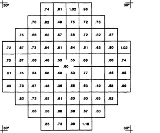
Normals: The variability o f the visual field in normal patients has been characterised in a
large study where subjects were randomly selected from a computerised population
database (Heijl et al. 1987). Using rigorous exclusion criteria, field data (Humphrey 30-2)
fcom 74 normals tested on 3 separate visits was obtained. Only data from the second and
third visits was used. From this data the intraindividual intertest variation and the
interindividual variation were calculated (Figure 5).
Figure 5 Intraindividual intertest variation - in dB.
Foveal variability -2.1 dB 5.6
4.9 5.2
4.9
4.3 4.9
4.6 4.7 4.2 3.7
2.9
3.4 3 .0
4.5 3.1 2.8 3.0
Peripheral variability -4.7 dB
3.4 4.3
2.2
3.3 2.3 3.5
5.0 3.4 2.4 2.1
4.7
2.4 3.7
2.3
4.2 2.7 2.3 2.0
2.1
5.2
2.1 3.3
2.3 1.6
5.6 2.2 1.9 1.8
6.1 3.5
2.4 3.9
4.3 3.0 2.4 1.8 2.4 2.2
4.3 2.3
2.7 2.4 2.4 2.5
3.0 3.4
3.0
4.2 3.7 2.4 2.4 4.2
5.8
4.8 5.0
4.9