Multiexponentiation Algorithm
Haimin Jin1,2
, Duncan S. Wong2?, Yinlong Xu1
1 Department of Computer Science
University of Science and Technology of China China
[email protected], [email protected] 2 Department of Computer Science
City University of Hong Kong Hong Kong, China
Abstract. Recently, a fast modular multiexponentiation algorithm for computing
AXBY (modN) was proposed [15]. The authors claimed that on average their
al-gorithm only requires to perform 1.306k modular multiplications (MMs), wherekis the bit length of the exponents. This claimed performance is significantly better than all other comparable algorithms, where the best known result by other algorithms achieves 1.503k MMs only. In this paper, we give a formal complexity analysis and show the claimed performance is not true. The actual computational complexity of the algorithm should be 1.556k. This means that the best known modular multiex-ponentiation algorithm based on canonical-sighed-digit technique is still not able to overcome the 1.5kbarrier.
Keywords: modular multi-exponentiation, modular arithmetic, canonic signed-digit representation, Hamming weight, Markov chain.
1 Introduction
Modular multi-exponentiation is an arithmetic operation that on input integers (x1,· · ·, xl), (e1,· · ·, el) and n, computes Qli=1x
ei
i (modn) for l > 1. This
oper-ation has been used in many number-theoretic cryptosystems [4,12,2,14] and the efficient implementation of this operation is very important to the performance of those cryptosystems as multi-exponentiation is one of the most expensive operations for them.
Fast algorithms for performing modular multiexponentiation are especially im-portant whenl= 2, that is, given integersA,B,X,Y andN, compute C=AXBY
(mod N). Digital Signature Algorithm (DSA) [7], ElGamal digital signature scheme [4], Schnorr’s signature scheme [12], Camenisch-Shoup public key encryption scheme [2], Waters’ identity-base encryption [14] and many other cryptographic algorithms
require to perform modular multiexponentiations forl= 2. However, modular multi-exponentiation is generally a very time-consuming arithmetic operation. To compute
C = AXBY (mod N), the traditional method is to solve the modular
exponentia-tions of AX (modN) and BY (modN) individually first and then multiply them together (followed by a modular reduction). This method is not optimal, even if one uses an optimal algorithm for the computation of AX (modN) and BY (modN).
Any improvement on the computational complexity of this operation will immedi-ately result in improving the performance of many cryptographic algorithms and protocols.
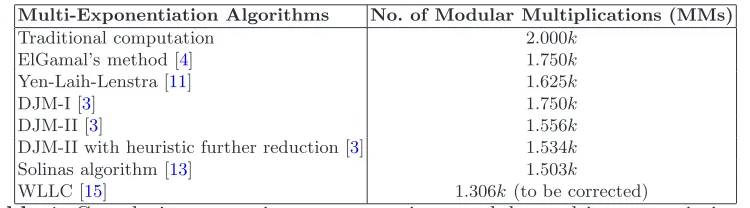
There have been many algorithms proposed [4,11,3,13] for performing fast mod-ular multiexponentiation. Among them, Canonic Signed-Digit (CSD) representation technique has been commonly used. In [3], Dimitrov, Jullien and Miller proposed two algorithms, which we call them as DJM-I and DJM-II. The expected number of Mod-ular Multiplications (MMs) of these algorithms are 1.75k and 1.556k, respectively, where kis the larger bit length of the two exponentsX andY. Recently, Wu, Lou, Lai and Chang [15] proposed an improved algorithm (which is termed WLLC in our paper) of DJM-II by introducing a complement representation method into the original DJM-II algorithm. They also claimed that the expected number of MMs can be significantly reduced to 1.306k. Table 1 shows the performance of various modular multiexponentiation algorithms.
Multi-Exponentiation Algorithms No. of Modular Multiplications (MMs)
Traditional computation 2.000k
ElGamal’s method [4] 1.750k
Yen-Laih-Lenstra [11] 1.625k
DJM-I [3] 1.750k
DJM-II [3] 1.556k
DJM-II with heuristic further reduction [3] 1.534k
Solinas algorithm [13] 1.503k
WLLC [15] 1.306k(to be corrected)
Table 1. Complexity comparison among various modular multi-exponentiation al-gorithms when l= 2. kis the larger bit length of the two exponents.
weight at most k2 has the expected fraction of bits that are zero is about 23 which is interestingly the same if we consider all k-bit integers.
Paper Organization. In the next section, we define several useful mathematical terms. This is followed by the review of WLLC and an informal comparison with DJM-II in Sec. 3. In Sec. 4, the formal analysis of the computational complexity of WLLC is given. It also determines the expected fraction of zero digits of k-bit integers with Hamming weight ≤k/2. We conclude the paper in Sec.5.
2 Mathematical Preliminaries
2.1 Canonic Signed-Digit Binary Representation (CSDBR)
Let B be ak-bit integer. A signed-digit binary representation of B is in the form:
B =
k−1
X
i=0
di2i di ∈ {0,1,−1}. (1)
A Canonic Signed-Digit Binary Representation (CSDBR) is a unique signed-digit representation which has no consecutive nonzero bits. It is commonly used to increase the efficiency of computer arithmetic. There are proofs [10,16,1,8] showing that the expected fraction of bits of an integer in CSDBR that are zeros is about 2
3.
The Hamming weight of an integer B, denoted Ham(B), is defined to be the number of nonzero bits in B. It has been well-studied with efficient algorithms available for finding the CSDBR, which gives the minimal Hamming weight among all the binary representations. From the fact above, on average, the Hamming weight of a k-bit integer in CSDBR is about k3.
2.2 A Signed-Digit Complex Arithmetic
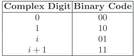
Gaussian integers are complex numbers of the form a+bi, where aand b are inte-gers. In 1989, Pekmestzi [9] introduced the following “binary-like” representation of Gaussian integers:
z=X
j
dj2j dj ∈ {0,1, i,1 +i}. (2)
This can be considered as a binary representation with complex digits. The digit encoding is shown in Table 2.
As an example of using this representation, let z = 2845 + 4584i, then we have 2845 = (0101100011101)2, 4584 = (1000111101000)2 and z = (i,1,0,1,1 + i, i, i, i,1,1 +i,1,0,1). By employing the encoding method of Table2, we obtain the following “binary-like” representation of z:
Complex Digit Binary Code
0 00
1 10
i 01
i+ 1 11
Table 2.Digit Encoding of Complex Digits
3 Review of WLLC [15]
As mentioned in the Introduction (Sec.1), Wu, Lou, Lai and Chang [15] have recently proposed an improved algorithm of DJM-II. In this paper, we call their algorithm as WLLC. When comparing DJM-II and WLLC, the WLLC has a conditional com-plement operation added with the purpose of further reducing the Hamming weight of the exponents, so to reduce the total number of modular multiplications (MMs). They claim that by adding this conditional complement operation, the Hamming weight of the exponents (which are represented as a “binary-like” Gaussian inte-ger) can further be reduced and result in faster algorithm for computing AXBY
(mod N). For exponentsX andY such that the length of max(X, Y) is kbits long, the average number of MMs required in DJM-II is 1.556kwhile it is claimed in [15] that WLLC only requires 1.306k MMs on average.
Let (X)SD be the CSDBR of X and X the complement of X. Fig. 1 shows
the pseudo-code of the WLLC algorithm. Below is an example (cited from [15]) for illustrating how this algorithm works.
Example 1. Compute C = A248 B31
(modN), where X = 248 = (11111000)2, Y = 31 = (00011111)2 and k = dlog2(max(X, Y))e = 8. Since Ham(X) > k2
and Ham(Y) > k2, we set X = −(X)SD = −(0000100¯1) = (0000¯1001) and Y =
−(Y)SD =−(100¯100000) = (¯100100000), where ¯1 denotes −1. Therefore, the result
is:
C=A248B31 (modN)
=A11111000B00011111 (modN)
=A100000000−(0000100¯1 )−1B100000000−(100¯100000)−1 (modN)
=A100000000+(0000¯1001)−1B100000000+(¯100100000)−1 (modN)
=(A28B28modN)×(A0000¯1001B100100000¯ modN)×(A−1B−1modN) (modN)
(3)
The Hamming weight of the original X+Y i = (1,1,1,1 +i,1 +i, i, i, i) is 8. Af-ter the transformation described in Fig. 1, the Gaussian integer z = (−(X)SD) +
(−(Y)SD)i= (−i,0,0, i,0,−1,0,0,1) which contains only 4 non-zero digits.
Input:A,B,X,Y,N
Output:C=AXBY (modN) Step 1:Pre-compute
kx=dlog2(X)e;ky=dlog2(Y)e;k= max(kx, ky);
a1 =AB (modN);a2=A−1 (modN);a3=B−1 (modN);
a4 =A−1B (modN);a5=AB−1 (modN);a6=A−1B−1 (modN);
a7 =A2 k
(modN);a8=B2 k
(modN);a9=A2 k
B2k (modN).
Step 2: IfHam(X)> k
2 thensetX =−(X)SD;HWx= 1elsesetX =XSD;HWx= 0. If Ham(Y)> k
2 thensetY =−(Y)SD;HWy= 1elsesetY =YSD;HWy= 0.
LetX=Pkx
j=0xj2jandY =P ky
j=0yj2j forxj, yj∈ {0,1,−1}. Step 3:Set Gaussian integerz=X+Y i, that is,z=Pk
j=0zj2j, wherezj=xj+yji. Step 4:SetC= 1.
Forj=kdown to 0do
C=C×C (modN)
switch(zj)
case1:C=C×A (modN)
casei:C=C×B (modN)
case1 +i:C=C×a1 (modN) case−1:C=C×a2 (modN) case−i:C=C×a3 (modN) case−1 +i:C=C×a4 (modN) case1−i:C=C×a5 (modN) case−1−i:C=C×a6 (modN)
Step 5: If (HWx= 1 andHWy= 0)thensetC=a7×C×a2 (modN) If (HWx= 0 andHWy= 1)thensetC=a8×C×a3 (modN) If (HWx= 1 andHWy= 1)thensetC=a9×C×a6 (modN) Step 6:OutputC
Fig. 1. The WLLC Algorithm for ComputingAXBY (modN)
12 MMs1
for computingA0000¯1001
B¯100100000
(modN) and two more for computing the final product, that is,a9×(A0000¯1001B
¯
100100000
modN)×a6 (mod N).
3.1 A Comparison With DJM-II
We now compare the complexity of WLLC with that of the original DJM-II [3] which is reviewed in Fig.4, Appendix A. As we can see, forX = 248 = (11111000)2
and Y = 31 = (00011111)2, their CSDBRs are (X)SD = (10000¯1000) and (Y)SD =
(0010000¯1), respectively. Hence the Gaussian integer z = (1,0,0, i,0,−1,0,0,−i) and Ham(z) = 4. The reduction of the Hamming weight in DJM-II is also from 8 to 4. As a result, by using the original DJM-II, the number of MMs taken for Example 1 above is 12.
1 We ignore the MM for computing C = C×C (modN) when j =k since the value of C is
always equal to one at that moment. As a result, there are 8 MMs corresponding toC=C×C
(modN) forj=k−1,· · ·,0 (wherek= 8) and 4 MMs corresponding to the 4 non-zero digits in
Example 2. We now take a look at another example from the WLLC paper [15], which computes C = A248
B15
(mod N). Similarly, X = 248 = (11111000)2
and Y = 15 = (00001111)2. Since Ham(X) > k2 but Ham(Y) ≤ k2, we
com-pute −(X)SD = (0000¯1001) and YSD = (0001000¯1), and set the Gaussian
inte-ger z = (0,0,0, i,−1,0,0,1 −i). Hence Ham(z) = 3 which yields the total number of MMs taken for getting the result of C to be 13 (i.e. 11 MMs for computing
A0000¯1001
B0001000¯1
(mod N) and two more for computing the final product, that is,
a7×(A0000¯1001B0001000¯1 modN)×a2 (modN).
If DJM-II is used, it is easy to verify that the Hamming weight of the Gaussian integer z is 4 and therefore, the total number of MMs required for computing C is 12.
Remark 1. It is interesting to note that in both of the examples above, DJM-II performs better than WLLC. The conditional complement operation introduced in WLLC does not seem to further reduce the Hamming weight of the Gaussian integer
z in any significant way, if there is any, and sometimes, it may be offset by the two additional MMs for computing the final product.
In [15], the authors also give the computational complexity analysis for the WLLC algorithm, according to which, they claim that the average number of MMs is 1.306k, which is much more efficient than all the known algorithms, as shown in Table 1. In the next section, we show that the actual computational complexity should be 1.556kwhich is comparable to that of the original DJM-II algorithm.
4 Complexity Analysis
According to Fig.1, we can see that on average, the number of MMs taken by WLLC is
NW LLC ≈k+ (1−fk/2 2)k= (2−f 2
k/2)k (4)
when k is large, where fk/2 denotes the average fraction of zero digits in each of X and Y of the Gaussian integer z in Step 3 (Fig. 1). In Eq. (4) above, the first termkcorresponds to the total number of C=C×C (modN) evaluations in Step 4 (Fig. 1)2
. The second term (1−f2
k/2)k corresponds to the number of non-zero
digits in the Gaussian integer z which incurs the MM operations in the switch-case statement of Step 4 (Fig. 1). For large k, the two additional MM operations for obtaining the final product in Step 5 (Fig. 1) can be ignored. NW LLC is used to
measure the computational complexity of WLLC.
For finding the value of NW LLC, we need to determine the value of fk/2. Note
that although it has been shown [10,16,1,8] that the average fraction of zero digits 2 As before, we ignore the evaluation when j=ksince the value of C is always equal to one at
of the CSDBR of k-bit integers is 23, this does not imply that the average fraction of zero digits of the CSDBR of thesubset ofk-bit integers under the condition that their Hamming weight is at most k2 is also 2
3.
The subsections below are organized as follows. We first review a CSDBR encod-ing algorithm in Sec. 4.1. In Sec.4.2, we formalize the CSDBR encoding algorithm as a state machine under the Markov chain model. This will facilitate our evaluation of fk/2. Then, we determine the expected Hamming weight of the CSDBR of k-bit
integers with Hamming weight at most k/2 and this is the value offk/2. In Sec.4.3,
we compute the corrected computational complexity for WLLC, that is, the value of NW LLC.
4.1 A CSDBR Encoding Algorithm
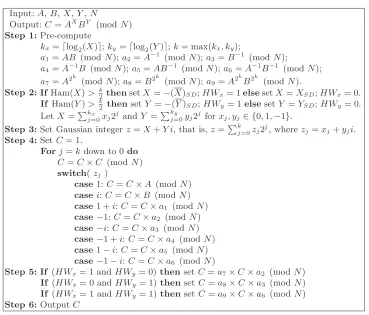
In Fig.2, we describe a CSDBR encoding algorithm which is derived from [1, Eq. (3)]. Let b= (bkbk−1. . . b2b1) be a k-bit integer (where bi ∈ {0,1}, for 1≤i≤k.
Input:b= (. . .0bk. . . bibi−1. . . b1)
Output:b= (. . . bibi−1. . . b1) — CSDBR ofb
0=· · ·=k+1:= 0 Fort= 1 tok+1do
If bt+t−1= 0 thensetbt= 0;t= 0 else if bt+t−1= 2thensetbt= 0;t= 1
else if bt+t−1= 1 andbt+1= 0thensetbt= 1; t= 0 else if bt+t−1= 1 andbt+1= 1thensetbt=−1;t= 1
returnb
Fig. 2. Arno-Wheeler CSDBR Encoding Algorithm
Let ˆbt be the generated CSDBR (i.e. the output bit of the algorithm) ofbt. We
can see that the algorithm in Fig. 2has four states as shown in Table 3.
State Condition ˆbt t
1 bt+t−1= 0 0 0
2 bt+t−1= 2 0 1
3 bt+t−1= 1;bt+1= 0 1 0
4.2 CSDBR Hamming Weight for k-bit Integers with Hamming Weight at Most k/2
The Arno-Wheeler CSDBR encoding algorithm reviewed in Table 3 has a set of four states S = {s1, s2, s3, s4}. The process of the Arno-Wheeler CSDBR encoding
algorithm starts in one of these states and moves successively from one state to another. Each move is called a step. If the chain is currently in state si, then it
moves to state sj at the next step with a probability denoted by pij, for some
1 ≤ i, j ≤ 4, and this probability does not depend upon which states the process was in before the current state. Therefore, the state transition satisfies the definition of a Markov chain. The probability pij is called transition probability. The process
can remain in the state it is in, and this occurs with probability pii. A transition
matrix can be composed accordingly. According to the state transition rules (see Table 3), we have Markov Chain Transition matrix as follows:
S =
1−a 0 a(1−a) a2
0 a (1−a)2
(1−a)a
1 0 0 0
0 1 0 0
(5)
where ais the probability that any bit equals 1. The stationary distribution is:
w= (w1, w2, w3, w4)
= ( (1−a)
2
a2−a+ 1, a2 a2−a+ 1,
a(1−a)2 a2−a+ 1,
(1−a)a2 a2−a+ 1)
(6)
The correctness of this distribution can easily be verified from the fact that wS=w
for all ergodic Markov chains ([6, Sec. 11.3]) and w1+w2+w3+w4= 1.
LetNk(j) be the frequency of state j (for j= 1,2,3,4 in Table3) that appears
in the CSDBR transition process. According to the Law of Large Numbers for Markov Chains ([6, Sec. 11.3]),Nk(j)≈wj∗k whenk→ ∞.
Since when j = 1 or 2, the output digit in CSDBR is zero, the fraction Zk of
zero digits in CSDBR is:
Zk=
Nk(1) +Nk(2)
k =w1+w2
= (1−a)
2
a2−a+ 1+ a2 a2−a+ 1
= 2− 1
a2−a+ 1.
(7)
Lemma 1. Let E(a) be the expected probability that a non-zero digit appears in a uniformly distributed k-bit integer with Hamming weight ≤ k/2. E(a) ≈ 1
2 when k→ ∞.
Proof. Let T be the number of k-bit integers with Hamming weight ≤ k2. Let i be the number of non-zero digits. Ci
k is the number of k-bit integers that have the
Hamming weight equal to i. 1. If k is odd, T = C0
k +C 1
k +· · ·+C
k−1 2
k . Since C 0 k +C
1
k +· · ·+C
k−1 2
k +C
k+1 2
k +
· · ·+Ck−1
k +Ckk= 2k, we have
T = 2k−1 (8)
2. Ifkis even,T =C0 k+C
1
k+· · ·+C
k 2
k. SinceC 0 k+C
1
k+· · ·+C
k 2−1
k +C
k 2
k +C
k 2+1
k +
· · ·+Ckk−1+Ckk, we have
T = 2
k+Ck2
k
2 (9)
Note that Cki/T denotes the fraction of the k-bit integers with i non-zero digits among all the k-bit integers with Hamming weight ≤ k2. Given i, for each of those
Cki integers with Hamming weight i, a non-zero digit appears with the probability
i
k. Hence the expected fraction of non-zero digits of any uniformly distributedk-bit
integers with Hamming weight ≤k/2 can be computed as follows:
E(a) =
bk 2c X
i=0 Cki
T · i
k (10)
According to [5, Eq. (5.18) on page 166], we know that
X
i≤m
Cki ·(k
2 −i) =
m+ 1 2 ·C
m+1
k (11)
By applying this to Eq. (10), we have
E(a) = 1
T·k[
X
i≤bk2c
Cki ·k
2 −
bk2c+ 1
2 ·C
bk2c+1
k ] (12)
1. Ifk is odd,T = 2k−1
, we have
E(a) = 1 2k−1·k ·
k
2 ·2
k−1
−b
k 2c+ 1
2k·k ·C
bk2c+1 k
≈ 1
2 (k→ ∞)
2. Ifk is even,T = (2k+C
k 2
k)/2, we have
E(a) = 1 2k+Ckk/2
2 ·k
·k
2 ·2
k−1
−
k 2 + 1
(2k+Ck/2 k )·k
·C
k 2+1
k
≈ 1
2 (k→ ∞)
(14)
For both of the approximations above, we use the fact that
lim
k→∞
Ckbk/2c
2k−1 = 0. (15)
u t
We now have the following theorem.
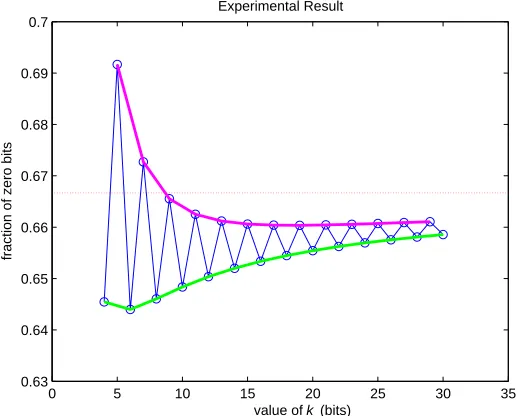
Theorem 1. For a uniformly distributed space constituted by all k-bit integers with Hamming Weight at most k/2, the expected fraction of zero digits in the CSDBR of integers in the space is 23.
Proof. According to Lemma 1, we have E(a) ≈ 1
2 (k → ∞). Then from Eq. 7, we
have that Zk= 23, when kis large. ut
Experimental Results. We have done an experiment to determine the average fraction of zero bits in the CSDBR of k-bit integers with Hamming weight at most
k/2. The experimental result is shown in Table4 and illustrated in Fig.3.
4.3 Computational Complexity of WLLC
Theorem 2. The computational complexity of WLLC for computing C = AXBY
(mod N) is about 1.556k when k is large, where k= max(dlog2(X)e,dlog2(Y)e). Proof. According to Theorem 1, the expected fraction of zero digits in the CSDBR of k-bit integers with Hamming weight ≤k/2 is 2
3. This is the value of fk/2, which
is the expected fraction of zero digits in each of X and Y of the Gaussian integer z
in Step 3 (Fig.1). Now from Eq. (4), we can compute the computational complexity of WLLC, that is, the value of NW LLC ≈(2−(23)
2
)k= 1.556k whenk is large. ut
5 Conclusion
We provided a formal complexity analysis and found that for the CSDBR of k-bit integers with Hamming weight ≤ k2, the expected fraction of zero digits is about 2 3
Lengthk Fraction Lengthk Fraction
4 0.645 5 0.692
6 0.644 7 0.673
8 0.646 9 0.666
10 0.648 11 0.663
12 0.650 13 0.661
14 0.652 15 0.661
16 0.653 17 0.660
18 0.654 19 0.660
20 0.65543 21 0.66044 22 0.65624 23 0.66057 24 0.65694 25 0.66073 26 0.65754 27 0.66090 28 0.65808 29 0.66107 30 0.65855
Table 4. Expected Fraction of Non-zero Digits in CSDBR of k-bit integers with Hamming weight ≤k/2
0 5 10 15 20 25 30 35
0.63 0.64 0.65 0.66 0.67 0.68 0.69 0.7
Experimental Result
fraction of zero bits
value of k (bits)
Fig. 3. Expected Fraction of Non-zero Digits in CSDBR ofk-bit integers with Ham-ming weight ≤k/2 — A Graphical Illustration
References
1. S. Arno and F. S. Wheeler. Signed digit representations of minimal Hamming weight. IEEE Transactions on Computers, 42(8):1007–1010, 1993. (Cited on pages3,6, and7.)
2. J. Camenisch and V. Shoup. Practical verifiable encryption and decryption of discrete loga-rithms. InAdvances in Cryptology - CRYPTO 2003, volume 2729/2003, pages 126–144. Springer Berlin, 2003. Lecture Notes in Computer Science. (Cited on page1.)
3. V. S. Dimitrov, G. A. Jullien, and W. C. Miller. Complexity and fast algorithms for multi-expontations. IEEE Transactions on Computers, 49:141–147, 2000. (Cited on pages2,5,12, and13.)
4. T. ElGamal. A public key cryptosystem and a signature scheme based on discrete logarithms.
IEEE Transactions on Information Theory, 31:469–472, 1985. (Cited on pages1and2.) 5. R. L. Graham, D. Knuth, and O. Patashnik.Concrete Mathematics. Addison-Wesley Publishing
Company, 1989. (Cited on page9.)
6. C. M. Grinstead and J. L. Snell.Introducation to Probability. American Mathematical Society, 1997. (Cited on page 8.)
7. ITL. Digital signature standard (DSS). Technical Report FIPS 186, National Institute of Standards and Technology, 1991. (Cited on page1.)
8. K. Koyama and Y. Tsuruoka. A signed binary window method for fast computing over elliptic curves. IEICE Trans. Fundamentals, E76-A:55–62, 1993. (Cited on pages3and6.)
9. K. Z. Pekmestzi. Complex number multipliers. InComputers and Digital Techniques, IEE Proceedings, volume 136, pages 70–75, 1989. (Cited on page3.)
10. G. W. Reitweisner. Binary arithmetics. Advances in Computers, 1:231–308, 1960. (Cited on pages3and6.)
11. S.-M.Yen, C.-S. Laih, and A. Lenstra. Multi-exponentiation. InComputers and Digital Tech-niques, IEE Proceedings, volume 141, pages 325–326, 1994. (Cited on page2.)
12. C. P. Schnorr. Efficient identification and signatures for smart cards. InAdvances in Cryptology - EUROCRYPT ’89, volume 434, pages 688–689. Springer Berlin, 1990. Lecture Notes in Computer Science. (Cited on page1.)
13. J. A. Solinas. Low-weight binary representations for pairs of integers. Technical Report CORR 2001-41, University of Waterloo, 1998. (Cited on page2.)
14. B. Waters. Efficient identity-based encryption without random oracles. In Advances in Cryp-tology - EUROCRYPT 2005, volume 3494/2005, pages 114–127. Springer Berlin, 2005. Lecture Notes in Computer Science. (Cited on page1.)
15. C.-L. Wu, D.-C. Lou, J.-C. Lai, and T.-J. Chang. Fast modular multi-exponentiation using modified complex arithmetic. Applied Mathematics and Computation, 186:1065–1074, 2007. (Cited on pages1,2,4,6, and11.)
16. C. N. Zhang. An improved binary algorithm for RSA.Computers and Math. with Applications, 25:15–24, 1993. (Cited on pages 3and6.)
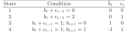
A Review of DJM-II
Fig. 4 shows the DJM-II algorithm [3]. In the algorithm, we recall that (X)SD
Input:A,B,X,Y,N
Output:C=AXBY (modN) Step 1:Pre-compute
kx=dlog2(X)e;ky=dlog2(Y)e;k= max(kx, ky);
a1 =AB (modN);a2=A−1 (modN);a3=B−1 (modN);
a4 =A−1B (modN);a5=AB−1 (modN);a6=A−1B−1 (modN) Step 2:setX = (X)SD andY = (Y)SD
LetX=Pkx
j=0xj2jandY =P ky
j=0yj2j forxj, yj∈ {0,1,−1}. Step 3:Set Gaussian integerz=X+Y i, that is,z=Pk
j=0zj2j, wherezj=xj+yji. Step 4:SetC= 1.
Forj=kdown to 0do
C=C×C (modN)
switch(zj)
case1:C=C×A (modN)
casei:C=C×B (modN)
case1 +i:C=C×a1 (modN) case−1:C=C×a2 (modN) case−i:C=C×a3 (modN) case−1 +i:C=C×a4 (modN) case1−i:C=C×a5 (modN) case−1−i:C=C×a6 (modN) Step 5:OutputC
![Fig. 4. DJM-II [3]](https://thumb-us.123doks.com/thumbv2/123dok_us/1861180.1241838/13.612.117.484.227.493/fig-djm-ii.webp)