TABLE OF CONTENTS:
Vol. 40, No. 4, July 1987
ARTICLES290 The Relationship between Land Ownership and Range Condition in Rich County, Utah by Michael W. Loring and John F. Workman
Grazing 294
299
303
307
310 315
318
322
330 333
336 339
342
A Dynamic Programming Application for Short-term Grazing Management Deci- sions by Abelardo Rodriguez and L. Roy Roath
Radiometric Reflectance Measurements of Northern Great Plains Rangeland and Crested Wheatgrass Pastures by J.K. Aase, A.B. Frank, and R.J. Lorenz Soil and Vegetation Responses to Simulated Trampling by Ahmed H. Abdel- Magid, M.J. Trlica, and Richard H. Hart
Soil Bulk Density and Water Infiltration as Affected by Grazing Systems by Ahmed H. Abdel-Magid, Gerald E. Schuman, and Richard H. Hart
Modeling Variation in Range Calf Growth under Conditions of Environmental Uncertainty by L.W. VanTassel], R.K. Heitschmidt, and J.R. Conner
l4-vs. 42-Paddock Rotational Grazing: Forage Quality by R.K. Heitschmidt, S.L. Dowhower, and J.W. Walker
Some Effects of a Rotational Grazing Treatment on Quantity and Quality of Available Forage and Amount of Ground Litter by R.K. Heitschmidt, S.L. Dowhower, and J.W. Walker
Responses of Fecal Coliform in Streamwater to Four Grazing Strategies by A. R. Tiedemann, D.A. Higgins, T.M. Quigley, H.R. Sanderson, and D.B. Marx
Cattle Grazing White Locoweed: Influence of Grazing Pressure and Palatability Associated with Phenological Growth Stage by M.H. Ralphs
Cattle Grazing White Locoweed: Diet Selection Patterns of Native and Introduced Cattle by M.H. Ralphs, L.V. Mickelsen, and D.L. Turner
Vegetation Recovery Patterns Following Overgrazing by Reindeer on St. Matthew Island by David R. Klein
Diet and Forage Intake of Cattle on Desert Grassland Range by Mark D. Hakkila, Jerry L. Holechek, Joe D. Wallace, Dean M. Anderson, and Manuel Cardenas
Seasonal Growth Rates of Tallgrass Prairie after Clipping by R.L. Gillen, and R.W. McNew
Range Improvement
346 Economic Returns from Treating Sand Shinnery Oak with Tebuthiuron in West Texas by D.E. Ethridge, R.D. Pettit, T.J. Neal, and V.E. Jones
348 Application of Herbicides on Rangelands with a Carpeted Roller: Timing of Treatment in Dense Stands of Honey Mesquite by Herman S. Mayeux, Jr. Plant Physiology
353 Nitrogen and Carbohydrate Partitioning in ‘Caucasian’and ‘WW-Spar’Old World Bluestems by B.I. Coyne and J.A. Bradford
361 Ecotypic Variation in Selected Fourwing Saltbush Populations in Western Texas by Joseph L. Petersen, Darrell N. Ueckert, Robert L. Potter, and James E. Huston Research Merhodology
367 Estimating Shrub Production from Plant Dimensions by H. Glenn Hughes, Larry W. Varner, and Lytle H. Blankenship
370 A New Sticky Trap for Monitoring Seed Rain in Grasslands by Laura Foster Huenneke and Courtney Graham
Published bimonthly-January, March, May, July, September, November
Copyright 1987 by the Society for Range Manage- ment
lNDlVlDUALSUBSCRlPTlONisbymembershipin INSTITUTIONAL SUBSCRIPTIONS on a calendar year basis are $56.00 for the United States postpaid and the Society for Range Management.
LIBRARY or other $66.00 for other countries, post- paid. Payment from outside the United States should be remitted in US dollars by international money order or draft on a New York bank.
BUSlNESSCORRESPONDENCE,concerningsub- scriptions, advertising, reprints, back issues, and related matters, should be addressed to the Manag- ing Editor, 1839 York Street, Denver, Colo. 80296. EDITORIALCORRESPONDENCE, concerning manu- scripts or othereditorial matters, should beaddressed to the Editor, 1639 York Street 86206.
INSTRUCTIONS FOR AUTHORS appear on the inside back cover of each issue. A Style Manual is also available from the Society for Range Manage- ment at the above address @$1.25 for single copies: $1.00 each for 2 or more.
THE JOURNAL OF RANGE MANAGEMENT (ISSN 0022-409X) is published six times yearly for $56.00 per year by the Society for Range Management, 1839 York Street, Denver, Cola. 80206. SECOND CLASS POSTAGE paid at Denver, Colo. POSTMASTER: Return entlre journal wlih address change-RETURN POSTAGE GUARANTEED-to Society for Range Management, 1839 York Street, Denver, Colo. 80206.
The Journal of Range Management serves as a forum for the presentation and discussion of facts, ideas, and philosophies pertaining to the study, management, and use of range- lands and their several resources. Accord- ingly, all material published herein is signed and reflects the individual views of the authors and is not necessarily an official position of the Society. Manuscripts from any source- nonmembers as well as members-are wel- come and will be given every consideration by the editors. Submissions need not be of a technical nature, but should be germane to the broad field of range management. Editor- ial comment by an individual is also welcome and subject to acceptance by the editor, will be published as a “Viewpoint.”
Managlng Edltor PETER V. JACKSON Ill
1639 York Street Denver, Colorado 80296 Edllor
PATRICIA G. SMITH
Society for Range Management 1839 York Street
Denver, Colorado 80206 Book Review Edltor GRANT A. HARRIS
Forestry and Range Management Washington State University Pullman, Washington 991646416
TECHNICAL NOTES
373 A Modified Sleeve and Plug Cannuln for Esophageal Fistuhted Cattle by J.F. Karn
375 An Updated Procedure for Cecal Cannulation in Sheep and Cattle by J.S. Caton, L.J. Krysl, AS. Freeman, J.L. Ruttle, and M.E. Branine
378 Use of Microsite Sampling to Reduce Inventory Sample Size by L.L. Larson and P.A. Larson
380 Allelopathic Effects of Kochia on Blue Grama by Moses Karachi and Rex D. Pieper
BOOK REVIEWS
382 Foundations for a National Biological Survey. Edited by Ke Chung Kim and Lloyd Knutson; The Ranchers: A Book of Generations by Stan Steiner; Arizona Soils by David M. Hendricks; Federal Public Land and Resources Law (second edition) by George Comeron Coggins and Charles F. Wilkinson; Federal Lands-A Guide to Planning, Management and State Revenues by Sally K. Fairfax and Carolyn E. Yale.
ASSOCIATE EDITORS G. FRED GIFFORD
Dept. of Range Wildlife, and Forestry University of Nevada
Rena, Nev. 89506 THOMAS A. HANLEY
Forestry Sciences Lab. Box 20909
Juneau, Alaska 99802 RICHARD H. HART
USDA-ARS 8408 Hildreth Rd. Cheyenne, Wyoming 82969 N. THOMPSON HOBBS
Colorado Div. of Wildlife 317 W. Prospect
Fort Collins, Colorado 80526 W.K. LAUENROTH
Department of Range Science Colorado State University Fort Collins, Colorado 86523 HOWARD MORTON
2ooO E. Allen Road Tucson, Arizona 85719
BRUCE ROUNDY 325 Biological Sciences East Building, Univ. Arizona Tucson, AZ 85721 NEIL E. WEST
Range Science Department Utah State University UMC 52 Logan, Utah 84322
LARRY M. WHITE USDA ARS
S. Plains Range Research Station 2WCl 18th St.
Woodward. Oklahoma 73801 RICHARDS. WHITE
USDA-ARS Route 1. Box 2021 Miles City, Montana 59301 STEVE WHISENANT
401 Widtsoe Building Brigham Young Univ. Provo, Utah 84662 JAMES YOUNG
USDA ARS
The Relationship between Land Ownership and Range
Condition in Rich County, Utah
MICHAEL W. LORINC AND JOHN P. WORKMAN Abstract
A study was conducted in Rich County, Utah, to determine the relationship between land ownership and range condition. Anrly- sis of variance and paired-plot t-tests were used to compare range condition ratings on Forest Service, Bureau of Land Management (BLM), state, and private lands. Forest Service land was in the highest range condition, BLM and private land had comparable intermediate condition ratings, and state-owned rangeland was in the lowest condition. Per acre grazing program expenditures in Utah by various hmd management agencies show an apparent correlation between expenditures and range condition. Thus, range condition may reflect management effort rather than the structure of public land property rights.
Key Words: range condition, land ownership, property rights structure, privatization
The relationship between land ownership (and associated prop- erty rights) and the use and health of renewable resources was an important focus in recent arguments to transfer federal land to private or state control. While the economic consequences of some such transfers have been addressed (Workman et al. 1981), there is little information concerning the impacts of ownership transfers on range conditions, long-term forage production, and erosion. Advocates of privatization suggest that the lack of efficient and well-defined property rights governing public land use has led to ecological degradation. They maintain that private ownership of natural resources is the only way to avoid resource depletion (Baden and Stroup 1977, Hardin 1977). Opponents of privatiza- tion contend that the market fails to address the public good of long-term ecological stability. They provide many historical examples to illustrate the short-sighted approach of the private sector and resulting mismanagement of western rangeland (Roset- ta 1985). Neither side, however, has offered comparable quantita- tive data to support their positions.
Some published information is currently available on the general condition of grazing land under the management of the Bureau of Land Management (BLM), Forest Service, and the private sector. Table 1 provides the percentages of grazing land in
Table 1. Percentages of total Utah rnngeland acreage in each range condi- tion class for each ownership.
Condition Class
Ownership class Excellent Good Fair Poor Other
Non-Fed’ 2 20 47 29 2
BLM* 4 33 39 16
USFS' - 27 46 27
USFP 13 36 37 14 -
‘U.S. Dept. of Agriculture, 1984a (SCS condition classification is: >75% climax vegetation q excellent, 51-75s = good, 2650% = fair, and 525% = poor). *U.S. Dept. of Interior, 1984(BLM condition classification is the same as that used by SCS).
W.S. Dept. of Agriculture, 1977 (USFS condition classification is: 61-100% climax vegetation = good, 41-60% q fair, 21-40s = poor, and Uo% = very poor). WSFS conditionclasses reported in 1977converted to SCSand BLM classificationas follows:excellent = l/2 USFSgood,good = 1/2X USFSgood + 1/2X USFSfair,fair = l/2 X USFS fair + l/2 X USFS poor, and poor = l/2 X USFS poor + very poor.
Authors are economist, Bureau of Reclamation, Salt Lake City 84147; and profes- sor of range economics, Range Science Department, Utah State University, Logan $4322. At the time of the research, Loring was a graduate research assistant, Range Science Department, Utah State University.
Published with the approval of the director, Utah Agricultural Experiment Station as Publication No. 3281.
Manuscript accepted I I March 1987.
290
each range condition class by major ownership categories for the state of Utah. While not providing statistical reliability, this table suggests that transfer of Forest Service grazing land to private ownership might, over time, result in a decrease in range condition. Range condition on BLM land also appears to be slightly better than on nonfederal rangeland. The limitations of this general condition information have been well explained in earlier reports (Box et al. 1976, Box 1979). Reliable conclusions cannot be drawn for 2 major reasons: (1) the general survey methods vary between agencies, as do sampling and estimation techniques; and 2) the sampling methodology for assessing range condition varies by agency and sampling year. In view of these limitations, we sampled a single representative county in Utah in order to achieve the statistical reliability needed for comparison of range condition among the different ownership classes.
Study Area
The area selected for study was Rich County, located in the northeastern part of the Utah panhandle (Fig. 1). Forest Service, BLM, Utah Division of State Lands and Forestry, and the private sector are well represented in the county, and all ownership groups manage grazing on large, contiguous acreages of rangeland. Eleva-
RICH COUNTY
r
USFS STATE ELM
PRIVATE I
I
/
I
I
I
/
Fig. 1. Mop of study Oreo. with regional orienrorion. showing land ownership.
tions range from 5,924 feet at Bear Lake to 9,148 feet at Monte Cristo Peak (Soil Conservation Service 1982). Sagebrush-grass communities dominate the 271,614 acres of rangeland (Utah Department of Agriculture 198 1). The sagebrush-grass ecosystem provides important spring and fall forage and is critical to the seasonal range use patterns of Rich County. Seven range sites comprising the majority of acreage within the sagebrush-grass ecosystem were selected for range condition evaluation. In addi- tion to economic importance, these range sites were selected because they readily exhibit vegetation composition responses to livestock use and demonstrate a consistent positive correlation between carrying capacity and range condition rating (Mason
1971). The 7 range sites, as identified by the Soil Conservation Service (1982), are: (1) mountain gravelly loam, (2) mountain stony loam, (3) upland loam, (4) upland shallow loam, (5) upland stony loam, (6) semidesert loam, and (7) semidesert stony loam.
Methods
The
experimental designs were an analysis of variance (ANOVA) randomized block design, using range sites as blocks and owner- ship classes as treatments, and a paired-plot sampling design ap- plied on range sites that extended across fence ownership boundar- ies for comparisons between ownership pairs.All soil mapping units in the county lying within the 7 selected range sites were identified through the use of the SCS soil survey guide (SCS 1982). Areas where grazing was not discretely con- trolled (i.e., state school sections and areas with checkerboard ownership configurations) were eliminated from the study. The soil mapping units were then numbered separately for each of the 2 experimental designs by range site and by ownership class or pair. Mapping units were selected for field sampling through random generation of their identity numbers. Three soil mapping units for each range site and each ownership class were sampled for the ANOVA test. The paired-plot test required sampling the same soil mapping unit on either side of a fenced ownership boundary. Each combination of range site and ownership pair was presented by 2 mapping units for the paired-plot test. A separate randomization scheme was used for the paired-plots to maintain design indepen- dence.
Sampling points were located at the approximate center of each randomly selected range site and the position marked on topogra- phical maps. Range sites dominated by introduced seeded species or small grain cultivation were eliminated and replacement sites were located through the previously described randomized scheme. The number of necessary relocations for each ownership class was recorded.
Field sampling was conducted from early June to early August in 1985. To minimize intra-seasonal variation, sampling began at lower elevations and proceeded to higher elevation sites as the season advanced. Two lOO-meter transect lines were extended at right angles from each sampling point and the orientation of the lines was randomly determined. Ten 0.5m2 circular plots were randomly located along each transect. Green weights for each species at each of the 20 circular plots were determinated using the double sampling method for weight estimation (Pechanec and Pickford 1937). A subset of 4 randomly selected plots were clipped for regression adjustments of weight estimates. Samples of each plant species at each sampling location were collected for conver- sion from green to dry-weights.
Range condition rating estimates were based on calculated spe- cies composition percentages using the standard SCS method (SCS 1976). Although it is recognized that the concept and mea- surement of range condition is currently being revised (Range Inventory Standardization Committee 1983), potential natural community indices and updated mapping units were not yet avail- able for Rich County. For this reason, SCS climax composition guides were used to rate range condition.
Some blocks of observations were not available, complicating
the statistical analysis of the ANOVA results. For example, the Forest Service boundary did not extend to lower elevation semi- desert sites, while the Utah Division of State Lands and Foresty did
not control grazing on higher elevation mountain sites (Table 2).
Table 2. Range condition ratings (percent climax vcgetetion) for ANOVA experimental design.
Range
Site
Number I.
Range Site
Mtn. Gravelly Loam
2. Mtn. Stony
Loam
3. Upland
Loam
Soil Mapping Units by Ownership Class
State Private BLM USFS
28 24 24
23 II 22
23 29 28
32 35 44
51 34 55
38 30 47
33 41 52
60 52 36
19 48 40
4. Upland Shallow 46 47 36 34
Loam 41 40 35 43
40 40 39 48
5. Upland Stony 26 34 17 33
Loam 34 29 31 35
29 26 44 28
6. Semidesert 46 53 49
Loam 55 60 53
55 41 46
7. Semidesert 36 63 47
Stonv Loam 23 51 47
43 38 38
For this reason, analyses of the 2 main effects of ownership class and range site, as well as the analysis of the interaction effect, were based on 3 data subsets from the principal design (Table 3). Aver- age range condition ratings for the ownership classes for each data subset were then compared using Least Significant Difference (LSD) confidence intervals @<.lO) based on the difference between 2 means (Neter and Wasserman 1974).
Table 3. F-test results for data subsets of the ANOVA design.
Number P Level
of of
Range Signifi-
Subset Sites Comparison Source F ratio cance A 4 Priv. vs BLM Ownership (0) 2.64 0.09
vs USFS Range Site (R) II.09 0.00
OXR 0.83 0.56
B 7 Priv. vs. BLM Ownership (0) 3.46 0.07 Range Site (R) 8.38 0.00
OXR 0.22 0.97
C 5 St. vs Priv. vs Ownership (0) 1.30 0.29 BLM Range site (R) 6.31 0.00
OXR 0.68 0.71
The paired t-test (significance set at 6.10) was used in the statistical analysis for the paired-plot design. It was not possible to directly compare Forest Service and state-owned lands because there were no adjacent tracts owned by these 2 agencies in Rich County.
Results
Range condition ratings for the ANOVAdesign are presented in Table 2. The 3 data subsets used for statistical analysis are as follows: Subset A (range sites 1,2,4, and 5) was used to compare
private, BLM, and Forest Service land; Subset B (all 7 range sites) was used to compare private and BLM land; Subset C (range sites 3 through 7) was used to compare state, private, and BLM land.
Although range condition ratings were significantly influenced by range site blocks (Table 3), pair-wise comparisons of block means revealed no recognizable trends. Significant mean differen- ces within an elevational grouping (i.e., mountain, upland, and semidesert) occurred as often as significant differences among elevation groups. Pair-wise comparisons also showed no apparent effect due to loamy, shallow, or stony soil characteristics. Inconsis- tencies in the percentages of plant species counted toward climax in the SCS technical guides may have contributed to this unclear effect. However, further analysis was not pursued because there was no significant interaction between range site and owner- ship (Table 3).
Data subsets A and B demonstrated a significant (pC. 10) rela- tionship between ownership class and range condition (Table 3). Further analysis of these subsets using pair-wise comparison (Table 4) showed that Forest Service range condition ratings were significantly higher @<. 10) than those for BLM land (Subset A). When all 7 range sites were examined (Subset B), private rangeland was also in higher condition than BLM land. Though not statisti- cally significant, private land also tended to be in higher condition than state land.
Table 4. Results of LSD pair-wise comparison of mean difference for data subsets of the ANOVA design.
Number of
Range Owner- Pair
Subset Sites Comparison ship Mean Comparison A 4 Priv. vs BLM Priv. 35.08 Priv. vs BLM
vs USFS BLM 30.42 Priv. vs USFS USFS 36.75 BLM vs USFS* B 7 Priv. vs BLM Priv. 41.33 Priv. vs BLM*
BLM 36.81
C 5 St. vs Priv. vs State 39.07 St. vs Priv. BLM Priv. 44.20 St. vs BLM BLM 40.67 Priv. vs. BLM *Significant at p<. IO
Paired t-test comparisons showed a stronger relationship between range condition and ownership class than did the ANOVA tests (Table 5). Forest Service rangeland was in higher (p<.lO) range condition than either private or BLM lands. However, there was no significant difference between the condition of BLM and pri- vate rangeland in the paired-plot experiment. Range condition on private land was significantly higher than on state-owned range-
Table 5. Summary of results for tbe paired-plot design.
Pair
Priv. vs. USFS
Priv. vs BLM
USFS vs BLM
Priv. vs St.
Ownership Mean Priv. 29.38 USFS 34.88 Priv. 37.60 BLM 38.60 USFS 39.50 BLM 38.20 Priv. 42.50 St. 35.60
Sample P level of Size t Significance
8 1.91 0.10
*o 0.21 0.84
8 3.87 0.01
1o 1.87 0.09
BLM vs St. BLM 50.33 3
1.84 0.21 St. 34.67
land, a result consistent with the results of the ANOVA pair-wise comparison. Although there was a large apparent difference between average condition of BLM and state rangeland, it was not statistically significant, due in part to an unavoidably small sample size.
Different sampling strategies of the 2 experimental designs explains why a stronger relationship between ownership and range condition was demonstrated by the paired-plot analysis than by the ANOVA. The minor differences in slope, aspect, and soil character change soil mapping unit delineations but do not affect SCS delin- eation of range sites. Samples in paired-plot comparisons involved the same soil mapping unit for each ownership pair, effectively removing all sources of variation other than ownership class. Thus, the paired-plot design is more accurate in detecting differences between ownership groups. NO contradictory outcomes were generated by the 2 experimental designs.
Discussion and Conclusions Land Transfer Impkations
The relationship between ownership class and range condition in Rich County corresponded closely with the information for Utah in Table 1. Forest Service rangeland was in higher condition than either BLM or private land. Thus, any transfer of Rich County Forest Service grazing land to private ownership might bring a decline in range condition. The higher condition of Forest Service rangeland compared to BLM land may reflect the historical fact that the Forest Service acquired control of livestock grazing sev- eral decades before the BLM (Wagner 1978). It is more difficult to predict the effects of privatization of BLM rangeland for several reasons. First, even though results of the ANOVA indicated that private rangeland was in higher range condition than BLM land, this conclusion was not supported by the more conservative paired r-test analysis.
Second, the statistical analysis did not consider how historical regulation of grazing has affected present condition of BLM range- land. As was noted in Senate Document No. 199 (U.S. Senate 1936), the most severe ecological degradation prior to the 1934 Taylor Grazing Act occurred on public domain rangeland that BLM later acquired. Thus, the fact that range condition of Rich County BLM lands is currently comparable to that of private rangelands might or might not be a valid argument against pro- posed privatization of BLM lands.
Finally, BLM and private range managers have different man- agement objectives. Twenty-nine percent of the sample sites ran- domly located on private rangeland had to be relocated due to seedings of crested wheatgrass (Agropyron crisrarum (L.) Gaertn.) monocultures, while only 1% of BLM sites were relocated for this reason. Therefore, transfer of Rich County BLM land to private ownership might bring increased seedings of non-native monocul- tures, an ecological change that should be considered.
The Effect of Property Rights
Comparisons of range condition on federal and private lands in Rich County were different than expected, based on incentive theory of renewable resource use. Resource economists contend that efficient user incentives occur only when all benefits and costs of using the resource accrue solely to the user (Tietenberg 1984). Although it is argued that this exclusivity requirement is not met by federal land grazing permits, other factors affecting range condi- tion may be more important than nonexclusivity. Change in range condition is a subtle and continuous process involving complex changes in the composition of plant communities. Sensitivity to these changes, which depends on available budget and expertise, can greatly affect range condition. The confounding influences of management objectives, expertise, budgetary allocation, and enforce- ment capability may have overshadowed the effect of illdefined federal property rights. Consequently, any proposal for federal land privatization based solely on the expected influence of prop- erty rights on user incentives seriously oversimplifies the situation.
Table 6. Comparison of agency expenditures on grazing programs in Utah for 1984.
Agency USFS BLM’ State of
Utah-’
1984 Expenditures Total Acres’ 1984 for Grazing Program($) Managed $/ac.
2,198,800* 7,990,7 lo-’ 0.275 3,331,969 22,708,363 0.146 228,000 3,785,296 0.076
306,000 0.081
lTotal acreages are used for consistency W.S. Dept. of Agriculture, 1984b ‘U.S. Dept. of Agriculture, 1985 ‘BLM, 1982 and 1985
,Utah Auditor General 1986 report to the Utah legislature on grazing program income for fiscal 1984. (Includes high and low estimates).
Even though property rights had less effect than other factors, this does not imply that property rights are not important. The comparison of private rangeland and Utah Division of State Lands and Forestry rangeland illustrates how property rights affect range condition. The goal of the State Lands and Forestry Division is to allocate the use of state lands to activities promising the highest returns to the state. Programs supervised by the State Lands and Forestry Division are accountable to the Utah Legislature Auditor General’s Office (Utah Auditor General report to Utah legislature 1985). Consequently, the range conservation objective is often secondary to that of generating income. Twenty-seven percent of the randomly selected sample sites on state-owned rangeland had to be relocated because they were in dryland wheat production, with some cultivation observed on soil mapping units with slopes averaging about 20% (SCS 1982).
The income-generating goals of the State Lands and Forestry Division may create strong incentives to not invest budget and labor in long-term improvements of range condition. Table 6 compares grazing program expenditures for the Forest Service, BLM and State of Utah. Relative per acre expenditures of the agencies follow the same pattern as the range condition ratings discussed above. The apparent correlation between grazing pro- gram expenditures and range condition among the agencies indi-
cates that the level of management effort may be more important than the effects of public land property rights.
Range condition comparisons between Rich County private and state lands conformed more closely to expectations based on prop- erty rights incentive theory. Because per acre grazing management expenditures were small on state lands (compared tofiderullands), state management effort had less confounding influence on the relationship between publicland propertyrightsand range condition.
Literature Cited
Baden, J., and R. Stroup. 1977. Property rights, environmental quality and the management of national forests, p. 229-240. In: Garrett Hardin and John Baden (eds), Managing the Commons. W.H. Freeman and Com- pany, San Francisco, Calif.
Box, T.W. 1979. The American rangelands: Their condition and policy implications for management, p. 18-27. In: Rangeland Policies for the Future. U.S. Dep. Agr. Policy Symposium Proceedings. Tucson, Ariz. Box, T.W., D.D. Dwyer, and FM Wagner. 1976. The public range and its
management. Report to the President’s Council on Environmental Qual- ity. March 19, 1976.
Bureauof Land Management. 19112. BLM facts and figures for Utah, 1982. Utah State Office. Salt Lake City, Utah.
Bureau of Land Management. 1985. BLM facts and figures for Utah, 1985. Utah State Office. Salt Lake City, Utah.
Hardin, C. 1977. An operational analysis of responsibility, p. 66-75. In: Garrett Hardin and John Baden (eds), Managing the Commons. W.H. Freeman and Company, San Francisco, Calif.
Muon, Lamar R. 1971. Yield and composition of Utah’s range sites. Soil Conservation Service, USDA. Salt Lake City, Utah.
Neter, John, and William Wassemun. 1974. Applied linear statistical models. Richard D. Irwin, Inc., Homewood, III.
Pechanec, J.F. and G.D. Pickford. 1937. A weight estimate method for determination of range or pasture production. J. Amer. Sot. Agron. 29:894-904.
Range Inventory Standardization Committee. 1983. Guidelines and termi- nology for range inventories and monitoring. Society for Range Man- age&&t, Denver, Colo.
Rosetta. Noel. 1985. Herds. herds on the Range. The Sierra Club Bulletin 7OL43-47.
Soil Conservation Service. 1976. National range handbook. USDA. U.S. Gov. Printing Office. Washington, D.C.
Soil Conservation Service. 1982. Soil survey of Rich County, Utah. USDA. U.S. Gov. Printing Office, Washington, D.C.
Tietenberg, Tom. 1984. Environmental and natural resource economics. Scott, Foresman and Company, Glenview, IIli.
U.S. Department of Agriculture. 1977. Region 4 summary of range condi- tion by states. Ogden, Utah.
U.S. Department of Agriculture. 1984a. Basic statistics, 1982. National Resources Inventory. SCS and Iowa State Univ. U.S. Gov. Printing Office, Washington, DC
U.S. Department of Agriculture. 1984b. Forest Service fiscal year financial summary data, Region 4. Ogden, Utah.
U.S. Department of Agriculture. 1985. Land areas of the national forest system as of September 30, 1985. FS-383. U.S. Govt. Printing Office, Washington, D.C.
U.S. Department of Interior. 1984.50 years of public land management. U.S. Gov. Printing Office, Washington, DC.
U.S. Senate. 1936. The Western Range. U.S. Senate Document 199,74th Congress, 2nd Session.
Utah State Department of Agriculture. 1981. Utah Agricultural Statistics. Salt Lake City, Utah.
Wagner, Frederick H. 19711. Livestock grazing and the livestock industry, py121-145 In: Howard P. Brodaw (ed), Wildlife in America. Council on Environmental Oualitv. U.S. Gov. Printing Office. Washinaton, D.C. Workman, John PI, E. &cc Godfrey, AllenD. LeBiron, ana D&win B.
Nielsen. 1981. Net economic costs of the proposed transfer of Utah’s federal lands to state ownership. Rangelands. 3:6-7.
A Dynamic Programming Application for Short-term Graz-
ing Management Decisions
ABELARDO RODRIGUEZ AND L. ROY ROATH Abstract
This study emphasizes short-term management decisions that are made in a yearling cattle operation in northeastern Colorado. Empirical equations describing forage and animal growth were coupled with marketing and supplementation rltemrtives. Four cases were modeled with high and low stocking densities and partial or total sales strategfes. Net present value of yearling steer sales were nuzhnized using dynamic programming.
Early sale of cattle was an economically favorable rltemrtfve
because of decreasing daily grins to-d the end of the grazing
season (September-October) and decreasing steer prices. Supple- mentation during September-October was also profitable to offset the decreasing trend in average daily gain caused by declining forage quality. Under the high stocking density and partial sales strategy, errly sales regulated standhtg crop left at the end of the grazing season. Under the low stocking density and partial sales strategy, early sales partially offset net return losses for those animals that had to be sold at the traditional marketing date. The total sales strategy favored sales of livestock 2 weeks before tradi- tional marketing under low and high stocking density and partial sales strategy. Net present values per pasture were slightly larger for the total sales strrrtegy than the partial sales strategy using both low and high stocking densities.
Key Words: yearling grazing, supplementation and marketing alternatives, optimal control application, net present value mazi- mization
Maximization of net returns or minimization of costs are major concernsin ranch management. In addition, considerations about cattle markets must be integrated into the net return equation. Accurate short term management decisions yield efficient forage utilization, high animal performance and profit maximization. Historically, most of the research done in range science decision models have dealt with long-term planning(Sharp 1967, Burt 1971, and Fisher 1985, among others) while short-term planning has been neglected (some exceptions are Bartlett et al. 1974, Hunter et al. 1976, Toft and O’Hanlon 1979).
This study emphasized the role of short-time decisions in forage and livestock management. The types of operation and manage- ment decision system employed were selected for their respective advantages. A yearling operation at the Central Plains Experimen- tal Range (CPER) was chosen for study because yearling opera- tions are more simply modeled and more sensitive to fluctuations in climate, forage quality, and market conditions than cow/calf operations. Dynamic programming (DP) was chosen over linear programming (LP) for various reasons:
1. The optimization problem can be defined in a free format (in contrast to matrix formulation needed for LP).
2. DP optimization can model nonlinear relations and does not require continuous functions to represent treatments. 3. While LP formulations increase in size to accommodate
piece-wise approximations of non-linear constraints, DP addresses such constraints directly.
Authorsare vistingassistant professor at the Department of Agricultural Econom-
ics, Oklahoma State University, Stillwater, T4074; and assistant professor at the Department of Range Science, Colorado State University, Fort Colhns 80523. At the time of the research the authors were graduate Student and assistant professor at the Range Science Department, Colorado State University, Fort Colhns 80523. This
study was done with financial support from fellowship No. 22313, National Council of Science and Technology (CONACYT) Mexico, and the Agricultural Experiment Station project No. 150781, Colorado State University. Larry Rittenhouse provided valuable help to develop the animal growth model. Thanks to Jonathan Trent, Tex
Lewis, and D.A. Jameson for reviews. Manuscript accepted 17 February 1987.’
294 -. ;
4.
5.
While multiperiod LP formulations require specifications of all possible values of the state variables for every period, DP narrows the solution space to specific values of state variables for different periods.
DP models may vary state variable growth rates. These rates
can be dependent upon previous state variable values, state variable interactions, and time. In contrast, serial LP models, such as the ones developed by previous authors (Sharp 1967, Bartlett et al. 1974, Hunter et al. 1976, and Propoi 1979), show production rates which vary only with respect to time. Dynamic optimization models yield a sequence of optimal deci- sion rules useful to decision makers (i.e., range managers). These optimal sequential rules make it possible to analyze marginal changes in biological or economic aspects of the cattle operation (van Poollen and Leung 1986).
Dynamic programming, an optimal control method, is not used extensively in range science because the implementation of optimal control theory and the algorithms to solve optimal control prob- lems are not well developed or widely understood (Trapp and Walker 1986). This paper will pursue a simple example of possible uses of deterministic DP in a yearling cattle operation.
Materials and Methods Data Sources
This study utilized data from the Central Plains Experimental Range (CPER) as input for the dynamic optimization model. CPER is located in northeastern Colorado as part of the shortgrass prairie of the Central Great Plains. Rolling hills separated by wide swales constitute its topography, and the soils include patches of loamy clay and loamy sand soils. Mean annual precipitation is 3 11 mm (70% of this falls between April and September), with annual extremes from 110 to 510 mm (Sala et al. 1981). The vegetation is dominated by blue grama (Boufelouu gracilis (H.B.K.) Lag.) and buffalograss (Buchloe dacryloides (Nutt) D.C.), constituting 65 to 9% of the forage grazed by cattle (Klipple and Costello 1960).
CPER’s yearling operation is typical of those in the Central Great Plains. Animals weighing 225 to 275 kg are bought in the spring, and are sold weighing 320 kg or more after grazing 3 to 5 months. Although this operation is typically a pasture program, this study considered supplementation with cottonseed meal as an alternative to offset a decrease in animal gains observed toward the end of the grazing season (Bement 1970).
Modeled Cases
Four cases were modeled with 2 selling strategies and 2 stocking densities (Table 1). In cases I and 2, half of the herd may be sold between 5 September and 17 October, with the remainder sold on 17 October 17 (traditional selling date). Cases 3 and 4 provide that half or all of the herd may be sold between September 5 and October 17, with the remainder of the cattle (if any) sold on October 17. The stocking density was 0.33 animals/ha (16 year- lings in a 48.6 ha pasture) for cases I and 3, and 0.49 animals/ ha (24 yearlings in a 48.6 ha pasture) for cases 2 and 4. The selected pasture size was not typical of yearling operations, but it could easily be adjusted to the pasture size of an existing ranch. Empirical equations for vegetation and animal growth were determined by regression analysis, and assembled into the DP model. A general- ized DP package (Labadie et al. 1982) was used to maximize net present value for the 4 cases previously described.
Table 1. The four cases modeled under different stocking densities and marketing str8tegiea.
Marketing Strategy
Partial Sales Total Sales
(half of herd may be (half or all of herd may sold between Sept. 5 be sold between Sept. 5 and Oct. 17 with and Oct. 17, with remainder sold on remainder (if any), sold
Oct. 17) on Oct. 17)
Low Stocking/Density
(I6 animals/48.6 ha) I 3
High Stocking Density
(24 animals/48.6 ha) 2 4
The Dynamic Optimization Model
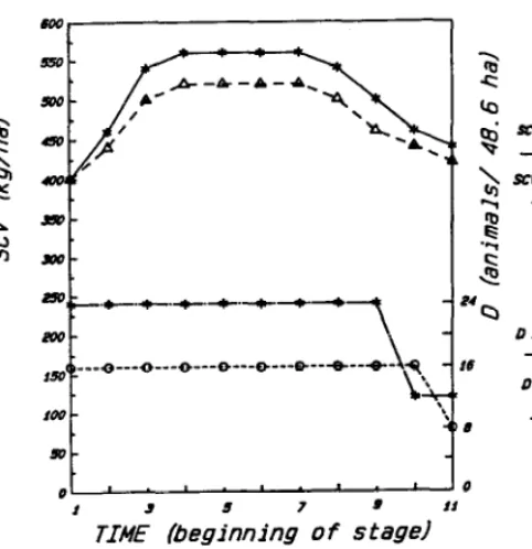
The model used here was dynamic in the sense that it optimized the sequence of decisions throughout the grazing season, in con- trast to static models that optimize over the entire grazing season. The dynamic optimization model had 3 variables: (I) standing crop of vegetation (SCV) ranging from 400 to 620 kg/ ha with 20-kg/ha intervals; (2) average animal weight (AWT) ranging from 235 to 350 kg with 5-kg intervals; and (3) number of animals per area (D) with 2 discrete values, 24 or 12 animals per 48.6 ha (high stocking density) and 16 or 8 animals per 48.6 ha (low stocking density). These discrete numbers are related to zero and 50% herd sales. Each of these state variables is related to 3 fundamental processes: forage growth, animal growth, and change in number of animals in the operation. Eleven stages were designated from late May to mid October. The beginning of stage 11 was only considered as the outcome of stage 10. A stage (subscript t) was defined as a 14-15 day period. At the beginning of that period, a decision (control u, defined below) was made and applied to the rest of that period (Fig. 1). Changes in number of animals depended upon the selling alternatives selected during the grazing season; these alternatives were considered in concert with supplementation alternatives. The DP recursive relation can be written as follows:
Ft(AWTt,SCVt,Dt) = Max ((Pit Yh. - TOTSUPPt P2, - VLABORJ u + BFt+l (AWTttl.SCVttlDt+l) - FOt) (1) where Pit and P2r were the steer prices in the Omaha market (USDA 1984)and cottonseed meal (USDA 1985)at stage t, respec- tively; TOTSUPPt was the weight of cottonseed meal fed to cattle during stage t (according to Bement 1970); VLABORtwas the cost of veterinary and labor expenses for stage t. This value was calcu- lated as 30 cents animal/day without supplementation, and 35 cents with supplementation*. Fixed outlay (FOt) was the initial cash paid for the steers (USDA 1984), this amount was zero for all stages other than 11 (beginning of the computational procedure). Fixed costs, such as land, were not considered. Ft was the maxi- mum net present value at stage t and Ft+l was the maximum accumulated net present value from previous stages where B was the discount factor based on 14% nominal annual interest rate.
Maximization in (1) utilized 5 different decisions (u) at each stage t:
When: u=l all livestock were marketed, u=2 livestock were supplemented,
u=3 the initial grazing scheme was maintained,
u=4 50% of livestock were marketed and the remaining animals were supplemented, and
u=5 5% of livestock were marketed and the remaining animals were not supplemented.
The quantity of livestock sold at stage t (Y&S
IC. Kerry Gee. United States Department of Agriculture, Economic Research Service, Department of Agricultural and Resource Economics, Colorado State University (personal communication).
following relation:
Y,,” = f (AWTtiD,,u) (2)
where Yt,” depended on number of animals per pasture (DS, the average weight (AWTS, and the decision u.
Average animal weight at stage t (AWTt) in equation 1 was defined by the following equation:
AWTt = AWTt-I + ADGt NODAYSt. (3)
Average animal weight in stage t depended on the average animal weight in the previous stage (AWTt-1) plus net animal growth (the product of the average daily gain at stage t (ADGS times the number of days (NODAYSS for that stage).
Average daily gain (kg per animal per day) at stage t was calcu- lated with the following equation:
ADG, = Z (-.895 + 902 RLNz+wr). (4)
Where Z was an adjusting factor for grazing conditions (dis- cussed below), and the relative limiting nutrient (Senft et al. 1984) for a specific weight (RLN,&r) was defined by the following expression:
RLNAw = Min (CPINT/ CP,, DEINT/ DEIll) . (5)
The minimum of 2 ratios, crude protein intake (CPINT) to crude protein for daily maintenance (CPS and digestible energy intake (DEINT) to digestible energy for daily maintenance (DEm). Daily intake and maintenance requirements (crude protein and digestible energy) for 250 to 400 kg steers gaining 0 to I kg of weight per day (NRC 1976) were used to estimate the linear function in paren- theses of equation 4. This equation was highly significant (Rzz.99, p<Ol) in predicting average daily gains for steers under feedlot
conditions.
Under grazing conditions, average forage intake (AVEINTt) was estimated with Conrad’s et al. (1964) equation multiplied by a linear decreasing function:
AVEINTt = (.0107 AWTJ (I-DMD)) G(AWTS. (6)
Where DMD was in-vitro dry matter digestibility of forage. According to Bourdon (1983), Conrad’s equation (first term in parentheses) underestimated the ratio fecal dry matter to live weight (.0107) in growing steers. To compensate for underestima- tion, G(AWTS was a linear decreasing function from 1.1 to 1.0, representing 10% extra forage intake for 235 kg steers and 0% for animals weighing 340 kg or heavier. Forage crude protein and in-vitro dry matter digestibility (Table 2) plus crude protein and
Table 2. Percentage of crude protein (CP) aad in-vitro dry matter dlgeati- bility (DMD) for tke gmzing aeason at CPER.
Period Stage CP DMD
5130 6/12 I 12.9 59.1
6113 6126 2 12.0 61.1
6127 7110 3 IO.8 59.5
7/ll 7124 4 9.8 56.9
7125 817 5 9.4 56.7
818 E/21 6 9.1 55.2
a/22 914 7 8.1 53.2
915 9119 8 7.1 51.1
9120 IO/3 9 6.8 51.7
IO/4 IO/ I7 10 6.5 52.2
Interpolated figures from monthly data reported in Dean and Rice (1975). Senft (1983), Uresk and Sims (1975) and Vavra et al. (1973).
Beginning
horizon.
of planning
May 30.
Stage - f4-15 daysForage utilizatibn is evaluated
Fig. 1. Temporalframework of the planning horizon and the sequence of stages in the DP.
dry matter digestibility of supplement (if provided), were used to calculate CPINT and DEINT. Daily maintenance requirements for crude protein and digestible energy were calculated with equa- tions provided in NRC (1976) to compute RLN*m. Subsequently, ADGtwas calculated only with the term in parentheses of equation 4. This equation underestimated average daily gains (without sup- plementation) reported by Bement (1968), Dyck and Bement (1971, 1972) and Senft (1983) at CPER. As a result, the constant Zz1.42 in equation 4 was an adjusting factor to grazing conditions at CPER. This constant was larger than 1, suggesting that steers with equal RLN value will gain more by grazing over feedlot conditions. The value of this constant can be explained by 2 arguments: (1) Animal selectivity affects CPINT and DEINT, and equation 6 did not imply that grazing animals select forage with higher quality than average; (2) According to Denham and Spreen (1986), NRC (1976, 1984) overestimates maintenance require- ments and underestimates efficiency in utilizing metabolic energy under high forage diets.
Standing crop of vegetation at stage t (SCVt) in equation 1 was defined by the following equation:
SCVt = SCVH + ANPPt - TOTINTt (7)
where ANPPt was the aboveground net primary productivity per stage t (kg/ha). This was defined as follows:
ANPpt q 14.44 + 4.098 PPTt-, + 1.726 PPTt - .174 SCvbl (8)
(Rz = .67,p<.Ol). Aboveground net primary productivity depended on precipitation (mm)during the previous and current stage (PPTt-1 and PPTt, respectively), as well as standing crop of vegetation in the previous stage (SCVt-1). Equation 8 was determined with biweekly data from Bement (1968) and Dyck and Bement (1971, 1972). Total intake at stage t (TOTINT*) in kg/ ha was defined as:
TOTINTt = AVEINTt D, NODAY&, (9)
296
horizon.
17.
where AVEINTt is average forage intake (kg per day per animal), Average forage intake was limited to 80%~ of estimated AVEINTtif a forage reserve level was lower than 380 kg/ ha as a consequence of forage overutilization. This condition defined a step function that related a threshold value of standing crop to animal intake, this assumed condition was used in the absence of empirical data for this relationship. Therefore, AVEINTt was dependent on the decreasing forage quality (DMD in Table 2) and possible shortage of forage (below the forage reserve level). In the absence of empiri- cal relationships that relate stocking densities and forage quality dynamics, this model assumed that stocking density per se did not exacerbate the temporal decreasing trend in forage quality.
Density of animals at stage t (Dt) in equation 1 was defined by the following equation:
Dt = Dt-1 -DdYt.S , WV
where the number of animals per pasture at stage t (Dt) was equal to the density of animals in the previous stage (Dt-1) minus the number of animals sold in stage t (DdYt,)).
Results and Discussion
Partial S&s Marketing Strategy
Cases 1 and 2 allowed partial sales at a given marketing date and utilized low and high stocking density, respectively. Optimal tra- jectories of the variables are described below.
Standing crop of vegetation followed similar trajectories for the 2 cases. During the first 3 stages there was a net increase in the standing crop (Fig. 2) corresponding to 97 mm of precipitation at CPER during that period (52% of the total rainfall during the grazing season). The standing crop of vegetation during the next 3 stages was stable while in the last 4 stages declined. The final standing crop of vegetation was 40 (low stocking density) and 20 (high stocking density) kg/ha above the initial 400 kg/ha at the beginning of the grazing season.
Under low stocking density, the number of animals per area during the first 9 stages was 16; at the beginning of stage 10 half of
::o
I 9TIMi
b9gjsnning'ofstage1
II
Fig. 2. Optimal trajectories of the state variables under partial sales strategy.
the animals were sold and 8 were kept to be marketed at the beginning of stage Il. Animals per area under high stocking den- sity were kept at 24 during the first 8 stages and decreased to 12 during stages 9 and IO. This suggested that greater grazing pressure prompted the decision to reduce the pressure one stage sooner than in the case of low stocking density. In order to avoid reduced forage intake and decreased animal growth, the stocking density was adjusted, resulting in partial sales.
Initial average animal weight was 235 kg. In both cases the average daily gain was 1.1 kg per animal per day during the first 3 stages, and later decreased to 0.7 1 kg per animal per day for the rest
#*op + m?mwlN - a%4orace8 L mm*lcoe
Fig. 3. Yearling steer price and average daily gain with respect to time.
JOURNAL OF RANGE MANAGEMENT 40(4), July 1987
of the grazing season, resulting in a final weight of 350 kg at the beginning of stage 11. Supplementation was .provided during stages 9 and 10 in both cases, preventing average daily gains of only .36 kg per animal per day.
Steer prices ($/cwt) in 1984followed the trend of the last 4 years (USDA 1984), as shown in Figure 3. Declining livestock prices towards the end of the grazing season must be taken into consider- ation since they affect net revenue. Using a low stocking density, livestock were sold early not because of forage overutilization but because it was more profitable to sell at stage 10 than stage 11. This was an economic decision based on the principle that additional revenue of retaining livestock one more stage must be larger or equal to the additional costs associated to that stage. This decision rule applies for discrete cases such as the ones presented here (i.e., the changes in returns and costs are calculated between stages or periods of time, as opposed to infinitesimal changes). For example, the revenue of selling steers at the beginning of stage 9 was $467.02 (330 kg divided by .454 kg/ pound multiplied by $64.25 and divided by 100 pounds); similarly, the revenues for selling cattle at stages 10 and 11 were $479.54 and $477.35, respectively. Total variable costs without supplementation at the beginning of stage 9 were $33.90, while total variable costs with supplementation the beginning of stages 10 and 11 were $39.36 and $44.44, respectively.
The difference between the change in revenues and the change in total variable costs between stages 9 and 10 was $7.06 (($479.54- 467.02)-($39.36$33.90)). The analogous difference between stages 10 and 11 was -57.27 (($477.35-$479.54)-(%44.44-$39.36)). At the beginning of stage 9 it was decided to retain the steers until stage 10 with $7.06 net return per stage; in contrast, at the beginning of stage 10 it was decided to sell the animals to avoid $7.27 net loss per stage. The net present value per 48.6 ha pasture at the end of stage 10 was $1,437 and $2,160 for low and high stocking densities, respectively (Table 3).
Table 3. Net present value (S)l per 48.6 ha pasture at CPER under different marketing stategka and stocking densities.
Difference Marketing Strategy Between Total
Partial Sales Total Sales and Partial Sales2
Low 1437 1529
Stocking Density (Sf%,
High 2160 2293
Stocking Density (3?%)
‘These calculations did not consider rent for land. depreciation of machinery or land investments.
‘The values in parentheses art the percent differences between total and partial s&S strategies with respect to total sale strategy.
Total Sales Marketing Strategy
Cases 3 (low stocking density) and 4 (high stocking density) allowed all of the animals to be sold at a given marketing date. As in the cases with partial sales strategy, SCV had a similar trend for both stocking densities. Under high stocking density, the SCV at the beginning of stage 10 was 400 kg/ha, equal to the initial SCV (Fig. 4). Under this marketing strategy, the forage resource was utilized close to the threshold level of 380 kg/ha. The number of animals per area was constant until all animals were sold at the end of stage 9 for the 2 stocking densities.
Initial animal weight was 235 kg. Under both stocking densities, animal growth was 1.1 kg per animal per day during the first 3 stages, decreasing to 0.71 kg per animal per day in the remaining stages. Supplementation took place in stage 9, and final weight was 340 kg at the beginning of stage 10.
Steer sales at the beginning of stage 10 were determined by the
6W
,i , . , . , _ , _ , .
J 9 9 7 9
TIME
(beginning
of stage)
SCV - St&%jJng crop of veg6trtJm 0 - Number of mJm6Js p6r we6 SD - StockJng density
F D IOU iv ___*__.
Fig. 4. i&lima1 rrajecrories of rhe slate variables under roral sales srrategy. declining prices toward the end of the grazing season (Fig. 3), a similar situation to that under partial sales strategy and low stock- ing density. The net present value per 48.6 ha pasture at the beginning of stage 10 was $1,529 and $2,293 for low and high stocking densities, respectively (Table 3).
The difference in the net present value per pasture between total and partial sales strategies was larger for high stocking densities ($87=2,293-$2,160) than the difference in the net present value per pasture between total and partial sales strategies for low stocking densities ($58=%1,529-$1,437). These differences with respect to the net present values of the total marketing strategies were 3.8% in both stocking densities (Table 3). This percentage was a net return loss related to the retention of 5% of the herd at the end of stage 10 under the partial sales strategy.
Conclusions
The combination of decreasing yearling steer prices and declin- ing forage quality towards the end of the grazing season dictated early sales in spite of the possibility,of livestock growth. Supple- mentation offset the trend in decreasing average daily gain toward
the end of the grazing season. It was a selected control as long as gain in revenue compensated the increased total variable costs of retaining steers another stage.
Under high stocking density and partial sales strategy, early sale regulated end-of-season standing crop. Under low stocking density and partial sales strategy, early sale minimized net return losses for those animals that had to be sold at the traditional marketing date. The total sales strategy favored sales of steers 2 weeks before traditional marketing under low and high stocking densities. In all cases, except under high stocking density and partial sales strategy, decreasing steer prices determined the early sale of cattle. Net present values per pasture were slightly larger for the total sales strategy than the partial sales strategy using both low and high stocking densities.
298
Literature Cited
Bartlett,
E.T., G.R. Evens, and R.E. Bemcnt. 1974. A serial optimization model for ranch management. J. Range Manage. 27:233-239. Bement, R.E. 1968. Herbage growth rate and forage quality on shortgrassrange. Ph.D. Diss. Colorado State University.
Bement, R.E. 1970. Fall gains of steers fed cottonseed cake on shortgrass
range. J. Range Manage. 23: 199-201.
Bourdon, R.M. 1983. Simulated effects of genotype and management on beef production efficiency. Ph.D. Diss. Colorado State University. Burt, O.R. 1971. A dynamic economic model of pasture and range invest-
ments. Amer. J. Agr. Econ. 53:197-205.
Conrad, H.R., A.D. Pratt, 8nd J.W. Hibbis. 1964. Regulation of feed intake in dairy cows. I. Change in the importance of physical and physiological factors with increasing digestibility. J. Dairy Sci. 4754-62. Dun, R.E. and R.W. Rice. 1975. Energy and nitrogen flow through cattle
on the shortgrass prairie. Grassland Biome. U.S. internat. Biol. Pro- gram. Tech. Rep. No. 293.
Denham, S.C., and T.H. Spreen. 1986. Introduction to simulation of beef cattle production. p. 39-62.1n:T.H. Spreenand D.H. Laughlin. Simula- tion of beef cattle production systems and its use in economic analysis. Westview Press, Boulder, Colo.
Dyck, G.W., and R.E. Bement. 1971. Herbage growth rate, forage intake and forage quality in 1970 on heavily and lightly grazed blue grama pastures. Grassland Biome. U.S. Internat. Biol. Program. Tech. Rep. No. 94.
Dyck, G.W., end R.E. Bement. 1972. Herbage growth rate, forage intake and forage quality in 1971 on heavily and lightly grazed blue grama pastures. Grassland Biome. U.S. Internat. Biol. Program. Tech. Rep. No. 182.
Fisher, I.H. 1985. Derivation of optimal stocking policies for grazing in arid regions. I. Methodology. Appl. Math. Comp. 17: I-35.
Hunter, D.H., E.T. Bartlett, and D.A. Jameson. 1976. Optimum forage allocation throughchance-constrained programming. Ecological Model- ling 2:91-99.
Kiippie, GE., and D.F. Costello. 1960. Vegetation and cattle responses to different intensities of grazing on shortgrass ranges on the Central Plains. USDA Tech. Bull. No. 1216.
Labrdie, J.W., J.M. Sheffer, and D.G. Fontane. 1982. CSUDP general purpose dynamic programming code. Dep. Civil Engineering, Colorado State Univ.
National Research Council (NRC). 1976. Nutrient requirements for beef cattle. Nat. Acad. Sci. Washington, D.C.
National Research Council. 1984. Nutrient requirements for beef cattle. Nat. Acad. Sci. Washington, D.C.
Propoi, A. 1979. Dynamic linear programming models for livestock farms. Behavioral Sci. 24:200-207.
Sala, O.E., W.K. Lauenrotb, W.J. Parton, and M.J. Triica. 1981. Water status of soil and vegetation in a shortgrass steppe. Oecologia 48:327-33 1. Senft, R.L. 1983. The redistribution of nitrogen by cattle. Ph.D. Diss.
Colorado State Univ.
S&t, R.L., M.A. Stiiiweii,end L.R. Rittenhouse. 1984. Seasonal changes in nitrogen and energy budgets of cattle range. Amer. Sot. Anim. Sci. West. Sect. Proc. 35:2C&203.
Sharp, W.C. 1967. A dynamic programming model for evaluating invest- ments in mesquite control and alternative beef cattle systems. Texas A&M Univ. Texas Agr. Exp. Sta. Tech. Monogr. 4 (September). Toft, H.I., and P.W. O’Hanion. 1979. A dynamic programming model for
on-farm decision making in a drought. Rev. Market. and Agr. Econ. 47:5-16.
Trspp, J.N., and O.L. Walker. 1986. Biological simulation and its role in economic analysis. p. 13-37.In:T.H. Spreen and D.H. Laughlin (eds.), Simulation of beef cattle production systems and its use in economic analysis. Westview Press. Boulder, Colo.
Uresk, D.W., and P.L. Sims. 1975. Influence of grazing on crude protein content of blue grama. J. Range Manage. 28:370-371.
U.S. Depertment of Agriculture. 1984. Market news weekly summary and statistics. Livestock division. Agr. Marketing Serv. Washington, D.C. Vol. 49-52.
U.S. Department of Agriculture. 1985. Feed outlook situation report. Fds. 294-296.
Vavra, M., R.W. Rice, and R.E. Bement. 1973. Chemical composition of the diet intake, and gain of yearling cattle on different grazing intensities. J. Anim. Sci. 36:441-444.
Van Pooiien, H.W., and P. Lang. 1986. Analyzing the effect of changing feed-beef price relationships on beef production on management strate- gies in Hawaii: a dynamic programming approach. West J. Agr. Econ.
11:106-114.