A Comparison of Cryptanalytic Tradeoff Algorithms
Jin Hong · Sunghwan Moon
the date of receipt and acceptance should be inserted later
Abstract Three time memory tradeoff algorithms are compared in this paper. Specifically, the classical tradeoff algorithm by Hellman, the distinguished point tradeoff method, and the rainbow table method, in their non-perfect table versions, are treated.
We show that, under parameters and assumptions that are typically considered in theo-retic discussions of the tradeoff algorithms, Hellman and distinguished point tradeoffs per-form very close to each other and that the rainbow table method perper-forms somewhat better than the other two algorithms. Our method of comparison can easily be applied to other situations, where the conclusions could be different.
The analysis of tradeoff efficiency presented in this paper does not ignore the effects of false alarms and also covers techniques for reducing storage, such as ending point trun-cations and index tables. Our comparison of algorithms takes the success probabilities and pre-computation efforts fully into account.
Keywords time memory tradeoff·Hellman·distinguished point·rainbow table
1 Introduction
There are numerous security systems in use today that rely on passwords. Access to many contents on the network requires one to login with a password and many file formats today have security features that restrict access to the file until the correct password is supplied. These systems are usually based on a password hash technique, which is to store a one-way function image of the password in the file or on the system. Indeed, storing the password
Contact author: Jin Hong
JH was supported by Basic Science Research Program through the National Research Foundation of Ko-rea(NRF) funded by the Ministry of Education, Science and Technology(2012003379).
J. Hong
Department of Mathematical Sciences and ISaC, Seoul National University, Seoul 151-747, Korea E-mail: [email protected]
S. Moon
Department of Mathematics, Texas A&M University, College Station, TX 77843-3368, USA E-mail: [email protected]
in its raw form within the file one wishes to set access control to would be meaningless. Authentication of a user is performed by recomputing the one-way function image from a freshly supplied password and comparing the result with the stored password hash.
A time memory tradeoff algorithm attempts to recover the password from the knowledge of the one-way function image, with the help of a table created through pre-computation. The massive pre-computation that is required before the actual attack can be mounted is the largest barrier in applying the time memory tradeoff technique to any specific security sys-tem. However, the pre-computation cost is roughly proportional to the size of the password space and, since many users do not use strong passwords, the tradeoff attacker is free to choose a manageable set consisting of short or more likely passwords and decide to be sat-isfied with recovering only those passwords belonging to this set. Then the pre-computation requirement does not stand as an impenetrable barrier to the tradeoff attack.
It has long been known that properly salting a password can remove any realistic threats of the time memory tradeoff attacks. The security system concatenates a randomly generated string (salt) of sufficient length to the user-supplied password before computing the one-way function image. The salt value that was used is stored alongside the computed password hash so that it is available to the system for the one-way function re-computation whenever a user needs to be authenticated. The effective number of passwords is increased by the use of salts and this can increase the pre-computation requirement of a tradeoff attack to an unrealistic degree.
Nevertheless, the salting countermeasure is still not being used in many proprietary sys-tems and some syssys-tems are known to be using both the newer salted and the older non-salted versions of the security system simultaneously to remain compatible with older systems. Hence, the time memory tradeoff technique still remains a powerful tool against these vul-nerable password hash systems. Since human generated passwords will continue to be used for the foreseeable future, one would like to fully understand the powers and limitations of the tradeoff techniques.
There are a large number of tradeoff algorithm variants, and we will restrict ourselves to the three major tradeoff algorithms in this work. The first algorithm we study is the original tradeoff algorithm [14] devised by Hellman. The second algorithm is the distinguished point method, which is attributed to Rivest in [10]. The number of table lookups that are required by a Hellman tradeoff is significantly reduced in this slightly modified method. The final algorithm we consider is the rainbow table method [24], announced by Oechslin. The pre-computation table for this method is structurally different from the previous two versions.
Let us briefly mention some of the more notable tradeoff variants or techniques that we are not treating in this work. The first is the perfect table version of the distinguished point method [8]. This is a variant of the distinguished point method where some of the redundancies contained in the pre-computed tables are removed and replaced with non-overlapping data generated through additional pre-computation. The more efficient usage of storage leads to better performance during the actual attack, at the expense of higher pre-computation cost. The removal of redundancies is facilitated by the distinguished point technique and cannot be done as easily with the classical Hellman algorithm, but the rainbow table method also admits a perfect table version [24] naturally. The perfect table versions of tradeoff algorithms are of interest due to their better efficiency during the attack phase. How-ever, analyzing them at the accuracy level aimed for by the current paper is quite delicate, and is left as a subject of future study.
inputs that were used to create the multiple one-way function images that are supplied as inversion targets. This class of algorithms attracted attention as realistic attacks on stream-ciphers, but present-day streamciphers are designed to withstand these attacks. The most practical application of the tradeoff technique today is with the password hash systems and we will present the current work with this application in mind.
Even though a considerable portion of this paper is devoted to the performance analyses of the three major tradeoff algorithms, the main motivation for this work was to determine which time memory tradeoff algorithm is the best. Providing a fair and acceptable answer to this seemingly simple question is the ultimate goal of this paper.
It has been shown [3, 4] that, if we restrict ourselves to a certain class of algorithms, the explicit tradeoff algorithms that are known today already achieve the best tradeoff efficiency one can hope for, at least asymptotically. However, the measure of efficiency considered by this theory is only accurate up to a small multiplicative factor. In practice, experience seems to be a critical factor in deciding which algorithm to use, and researchers have varied opinions on which algorithm performs better.
Comparison of tradeoff algorithms has been a controversial subject. There are claims of superiority of one algorithm over another, but, in many cases, these are either heuristic arguments or based on complexity analyses that are not accurate up to small constant factors. There are at least two obstacles to providing a fair comparison of tradeoff algorithms. The first is that the online time of each algorithm is hard to predict accurately, due to certain events called false alarms. Some answers to this problem may be found in [1, 15] for the Hellman and rainbow cases. The current paper relies heavily on these results. The second obstacle concerns the minimal number of bits required to store each pre-computation table entry. In particular, a technique for storage optimization called ending point truncation has not yet been fully analyzed.
There is a naturally occurring measure of how efficiently a tradeoff algorithm balances time against storage in achieving its goal and the accurate value of this efficiency measure becomes accessible once the first obstacle mentioned above is resolved. As was first noted in [3, 4], the measure of tradeoff efficiency has been expressed in different units for different algorithms. In this work, by extending the approach of [3, 4], we carefully convert the trade-off efficiency measures for the three algorithm to a common unit so that they may directly be compared. The unification of units is intimately connected to the second obstacle mentioned above. We also carefully treat the time taken for table lookups during our initial transition of units.
The above two obstacles that are due to our lack of accuracy in presenting the trade-off efficiency figures can be overcome through rigorous algorithm analyses, but there is yet another problem which is related to the pre-computation cost. Currently there is no widely accepted way of comparing two algorithms that can achieve different tradeoff performances only after the investment of different pre-computation efforts. Due to this difficulty, many comparisons of tradeoff algorithms have focused on the above mentioned measure of bal-ancing capability and have ignored the cost of pre-computation.
pre-computation cost and tradeoff efficiency relative to each other, and, in most cases, the judgement cannot be done in an objective manner.
While presenting the above comparison method, we will mainly focus on a certain set of parameters and environmental assumptions that are typically considered during theoretic analyses of tradeoff algorithms. Under the circumstances under focus, the classical Hellman and the distinguish point methods are shown to perform very close to each other. When placed under the additional requirement that the success rates of the tradeoff algorithms must be high, the rainbow table method is shown to outperform the other two algorithms. These comparison conclusions will stand true for any relative valuing of the pre-computation cost and tradeoff efficiency, as long as we are working with the typical situation. Comparisons at other situations can easily be done by following through our methods, and the resulting conclusions can be different.
The remainder of this paper is organized as follows. In the next section, we fix notation and terminologies while reviewing previous results related to this work. Section 3 clarifies the connection between the theory of tradeoff algorithms and the use of the algorithms in attacking password hash systems. In Section 4, Section 5, and Section 6, we study the distin-guished point, Hellman, and rainbow table tradeoff algorithms, in turn. For each algorithm, we present an accurate tradeoff efficiency figure that does not ignore small multiplicative factors and also analyze the applicable storage reduction techniques. These sections over-come the first and second obstacles that were mentioned before. Comparisons of tradeoff efficiencies under different parameter sets for the same algorithm are made in Section 7. Finally, our goal of algorithm comparison is reached in Section 8, and the work is sum-marized in Section 9. Experiment data supporting the arguments of this paper are given in Appendix E. We acknowledge that a small part of this work was previously made public through [21].
2 Time Memory Tradeoff Algorithms
In this section we review the basic theory of time memory tradeoffs and fix notation that is used throughout the paper. We introduce previous results that are related to the results of this paper, but make no attempt at providing a complete history or survey of the time memory tradeoff technique. In particular, the perfect table tradeoffs algorithms are explained, but advancements concerning their analyses or comparisons are not introduced.
Below, after stating some simple technical facts, we describe the three major tradeoff algorithms, and then explain some auxiliary techniques that can enhance their tradeoff ef-ficiency. The descriptions are dense and readers that are new to the time memory tradeoff technique should consult the original papers for more detail.
Throughout this paper, the function F :N →N will always act on a setN of sizeN
and the k-times iterated composition F◦ · · · ◦F of F is written as Fk.
2.1 Technical preliminaries
set of all functions of certain domain and codomain. In other words, any expected value expressed for a random function is an average computed over all function.
For large positive integersaandbsuch thata=O(b), we can use the approximation
1−1b
a
≈ e−ab,
which is very accurate. For example, whena=b, the error in the approximation is bounded
by be. This approximation is frequently used in the tradeoff literature without any
expla-nation and is also used very frequently in this paper. Its use can be justified through easy computation, which is explicitly carried out in Appendix A.
The final technical fact we present concerns the image size of a random function. Let F :N →N be the random function. IfM ⊂N is of size m0, then the size of F(M)is expected to be
m1=N
n
1−1−N1m0o≈N 1−e−m0N. (1)
An elementary proof of this statement can be given by treating it as a classical occupancy problem.
More generally, the expected k-th iterated image size mk=E |Fk(M)|
can be itera-tively computed through
mj=N 1−e−
m j−1
N (j=1, . . . ,k), (2)
starting from m0=|M|. This is stated in [11, 20] to hold asymptotically. The explicit state-ments given there are only for the case when the input setM is the complete domainN,
but the case whereM is strictly smaller than the complete domain is used in [24] to state the success probability of a non-perfect rainbow table. The relation between (1) and (2) is carefully discussed in Appendix B.
2.2 Overview of the tradeoff technique
Let F be fixed to a publicly known one-way function. The goal of any tradeoff algorithm is to recover the input x, when it is given the function image y=F(x). The correct answer x and the inversion target y may occasionally be referred to as the password and password hash, respectively.
Any tradeoff algorithm consists of a pre-computation phase and an online phase. The pre-computation phase algorithm gathers information about the one-way function F through extensive computation and stores a condensed digest of the gathered information in a pre-computation table. The online phase is when the algorithm is given the target y=F(x)to invert and tries to recover x using the pre-computation table.
To be meaningful as an attack, the size M of the pre-computation table must be smaller thanNand the online phase algorithm should return the answer in time T that is shorterN.
Note thatN is the size of the complete dictionary {(x,F(x))}x
∈N and is also the time
Even though every implementation of the tradeoff technique works with a specific one-way function F, analyses of the tradeoff techniques are alone-ways done with the assumption that F is a random function.
2.3 Hellman tradeoff
The first algorithm we explain is the classical tradeoff algorithm by Hellman [14].
2.3.1 Parameter setup
Certain parameters need to be fixed before the pre-computation phase can be started. Positive integers m and t that satisfy the relation mt2≈Nare fixed. This equation is referred to as
the matrix stopping rule. Another positive integerℓ≈t, which will become the number of tables, is also fixed.
In this paper, we let the parameters m and t satisfy mt2=HmscN, with a matrix stopping
constantHmscthat is neither very large nor too close to zero. Much of the tradeoff literature setsHmsc=1. The conditions we have given toHmscandℓmay (inaccurately) be expressed as Hmsc=Θ(1)andℓ=Θ(t), respectively. The parameters are always assumed to be reasonable in the sense that 1≪m,t≪N. The tradeoff algorithms behave somewhat differently when
instantiated with extreme parameters.
The reduction functions Rk:N →N, one for each k=1, . . . , ℓ, are fixed. These may
be any family of simple bijections that are very easy to compute. WhenNis a power of 2 and N consists of non-negative integers less thanN, bit permutations or XOR-ing by constants
are practical choices for reduction functions. The colored iterating functions Fk:N →N
are defined through Fk=Rk◦F.
2.3.2 Pre-computation phase
In the pre-computation phase, what is explained below is repeatedℓtimes, once for each 1≤k≤ℓ, to buildℓtables.
We start by choosing m random starting points spk
1,spk1, . . .,spkm∈N. Hellman
speci-fied for each starting point to be chosen independently at random, but most researchers today see the starting points as being distinct. For each 1≤i≤m, we initially set xki,0=spki and
recursively compute xki,j=Fk(xik,j−1)for 0<j≤t. The final point reached by each chain of iterative computations is said to be an ending point epki =xki,t=Fkt(spki). The ordered pairs
{(spki,epk i)}
m
i=1 are stored as the k-th Hellman table, after being sorted with respect to the ending points.
The collection of all points {xki,j}i,j, associated with an iterating function Fk of one
color k, is said to be a Hellman matrix of size m×t. One usually visualizes a Hellman matrix as follows.
spk1=xk1,0 −−→Fk x1,1k −−→Fk xk1,2 −−→ · · ·· · ·Fk Fk
−−→ xk1,t−1 −−→Fk xk1,t=epk0 spk
2=xk2,0
Fk
−−→ xk
2,1
Fk
−−→ xk
2,2
Fk
−−→ · · ·· · · Fk
−−→ xk
2,t−1
Fk
−−→ xk
2,t=epk1 ..
. ...
spkm=xkm,0
Fk
−−→xkm,1
Fk
−−→xkm,2
Fk
−−→ · · ·· · · Fk
−−→xkm,t−1
Fk
It consists of m rows and t+1 columns. We number the columns so that the starting point column is the 0-th column and the ending point column is the t-th column. Each row of a Hellman matrix is a pre-computation chain. Any chain of points fromN that has been
formed by iteratively applying an Fkof the same color k is a Hellman chain.
2.3.3 Online phase
Once the inversion target y=F(x)is given, the process explained below is repeated for each 1≤k≤ℓ, until the correct answer x is found. Occasionally, the algorithm will report failure in returning the answer after processing allℓindices k.
We first compute yk1=Rk(y) =Fk(x)and check if this appears as one of the ending
points in the k-th Hellman table. The table lookup is repeatedly done for each recursively computed yk
j=Fk(ykj−1), until ykt =Fkt(x)has been searched for in the table. The Hellman
chain
x−−→Fk
yk1
Fk
−−→yk2
Fk
−−→yk3
Fk
−−→ · · ·· · · Fk
−−→ykj
that is computed through this process is referred to as the online chain for the k-th Hellman table.
Whenever a match yk
j=epki is found, the corresponding starting point spki is retrieved
from the k-th Hellman table, and the associated pre-computation chain is (partially) regen-erate to obtain xtmp=xki,t−j=F
t−j
k (sp
k i). Since
Fkj(xtmp) =Fkj(F t−j
k (sp
k
i)) =epki=ykj=F j−1
k (y1) =F
j k(x),
there is a chance that xtmp=x. This is why the j-th iteration of the online phase for a specific
table is sometimes referred to as searching for the answer x among the(t−j)-th column of the Hellman matrix. If multiple ending points match the current end of the online chain, one must not forget to regenerate all the corresponding pre-computation chains.
Even though the existence of x in the(t−j)-th column of a Hellman matrix will surely imply the collision of ykjwith an ending point, the converse is not true unless Fkis injective.
An ending point collision could be caused by a merge between the online chain and a pre-computation chain. Hence, the online phase algorithm must check whether the candidate answer xtmp is the correct answer x. The candidate is clearly incorrect if F(xtmp)6=y, but
a full verification requires more information than is contained in y and this is explained in more detail in Section 3. If the candidate xtmpis found to be incorrect, the event is referred
to as a false alarm, in which case the online phase resumes the iterative computations of the online chain.
2.3.4 Success probability
The algorithm description for the Hellman tradeoff is complete and we now give some rough analyses.
The success of inversion is intimately related to how many distinct points are covered by the Hellman matrices. Assume that there are not too many duplicates in an m×t Hellman matrix and consider the addition of one more pre-computation chain to this matrix. The ex-iting Hellman matrix and the new chain contain approximately mt and t points, respectively. Since the matrix stopping rule gives mt·t≈N, we know from the birthday paradox that there
much of the computation that was done to create this additional chain goes to waste. Hence, it makes little sense to continue enlarging a Hellman matrix beyond the m×t bound set through the matrix stopping rule. This is the reason for using multiple small tables, rather than a very large table. The discussion given so far also indicates that the duplicates within the matrix will not be too many until one comes close to the m×t bound.
Let us use|HM|to denote the expected number of distinct nodes contained in a Hellman matrix. The probability of successful inversion after the processing of a single Hellman table is |HMN|. Hellman [14] provided the lower bound
|HM|
N ≥
1
N
m
∑
i=1
t
∑
j=1
1−Nitj (3)
and used it to explain the appropriateness of the matrix stopping rule. The arguments given above that involves the birthday paradox are from [5, 6], and may not be found in [14].
When allℓ≈t tables are processed, assuming that the reduction functions provide inde-pendence between tables, the probability of success becomes
1−1−|HMN|ℓ≈1−exp
−ℓ|NHM|. (4)
Since the number of duplicates within each Hellman matrix is kept low by the matrix stop-ping rule, we have|HM| ≈mt. Recallingℓ≈t and applying the matrix stopping rule, we can state that the probability of the Hellman tradeoff in successfully recovering the correct an-swer x is approximately 1−1
e≈63.2%. This is sufficiently large for the Hellman algorithm
to be meaningful as an attack.
Interestingly, the original paper [14] does not explicitly express the success probabil-ity (4) of the complete algorithm. It is only stated that the inverse of the right-hand side of (3) should be taken as the approximate number of pre-computation tables that are to be created. However, statements similar to (4) may be found in works as far back as [17, 18].
In [18], the right-hand side of (3) was carefully approximated, so that the bound could be rewritten as
|HM|
N ≥
mt
N
1 Hmsc
Z Hmsc
0
1−e−x
x dx. (5)
Experiment data provided in the work supports the correctness of this bound, but it also showed that this bound was far from being tight. For example, atHmsc=1, the test data provided was|HMN|=0.85
mt
N, while the right-hand side of (5) was 0.80
mt
N.
This discrepancy was resolved by [9, 19], which computed the expected value|HM|itself, rather than its lower bound. This result is copied as Proposition 21 in the main body of the current paper.
2.3.5 Cost of resolving alarms
An upper bound for the number of false alarms per table was given asHmsc
2 in [14]. This was combined with the fact that resolving each alarm requires at most t iterations to argue that the side effects of false alarms on the online time complexity was limited.
A much better bound on the effects of false alarms is given in [18] as
(cost of resolving alarms for all tables)≤Hmsc
6 ℓt. (6)
Almost the same content reappears in [15], expressed in the form
(expected cost of resolving alarms per table)=Hmsc
6 t. (7)
The proofs given by the two paper for the above two statements are essentially identical.
2.3.6 Tradeoff curve
We haveℓ≈t tables, each containing m entries, so that the total storage size is M=mℓ≈mt. Disregarding the time taken to treat false alarms, it takes t iterations of the one-way function to process each of theℓ≈t tables, so the online time complexity is at most T≈tℓ≈t2. Applying the matrix stopping rule to T and M, one can arrive at the trade-off curve
T M2≈N2 (8)
for the Hellman tradeoff.
Conversely, suppose that certain values T and M satisfy the trade-off curve (8). Then the parameters t=√T and m=M/√T satisfy the matrix stopping rule. When the Hellman tradeoff is implemented with these t, m, andℓ≈t, it will require storage M and run in online time T .
The tradeoff curve (8) did not appear in the original publication [14]. The above presen-tation has been adopted from [5, 6].
2.4 DP tradeoff
The distinguished point method, which we shall simply refer to as the DP tradeoff, is a simple modification of the Hellman tradeoff. Introduction of the DP technique is attributed to Rivest in the book [10], but no corresponding publication can be found. The perfect table version of the DP tradeoff was first studied in [7, 8] and this was followed by some further analyses in [1, 25, 29], but literature analyzing the non-perfect DP tradeoffs, which we deal with in this work, is hard to find.
2.4.1 Parameter setup
As in the Hellman tradeoff, one fixes positive integers m and t satisfying the matrix stopping rule mt2≈N. Reduction functions Rk:N →N are chosen and colored iterating
func-tions Fk=Rk◦F are defined as before. Our work will use the notation mt2=DmscNwith
One fixes a property which is satisfied by a random element ofN with probability 1t. This distinguishing property should be very easy to check. For example, suppose that t andN
are powers of 2 and that the setN consists of non-negative integers less thanN. Then, one
usually defines an element ofN to be a distinguished point , or a DP, if the first log t bits of
its binary representation are zero.
2.4.2 Pre-computation phase
Rather than fixing the length of each pre-computation chain to t, the pre-computation itera-tions xki,j=Fk(xki,j−1)are continued until the current chain end x
k
i,jis found to be a DP. The
resulting m pre-computation chains will be of varying lengths, but their average length will be t. As in the Hellman tradeoff, the m starting point and ending point pairs are stored as a DP table andℓtables are constructed, each corresponding to a different color 1≤k≤ℓ.
Any chain computed through iterative applications of a single Fk that ends at a DP is
a DP chain. The collection of all pre-computed DP chains associated with one DP table is referred to as a DP matrix, even though the collection can no longer be visualized as a rectangular shaped matrix.
2.4.3 Online phase
Given the inversion target y=F(x), the online phase of the DP tradeoff proceeds quite similarly to the Hellman tradeoff online phase. However, since only DPs can be found among the ending points, table lookups are done only when the iteratively computed yk
jis found to
be a DP. Since no pre-computation chain contains a DP in the middle part of the chain, the online chain iterations for any single DP table is terminated at its first DP occurrence.
Resolving alarms is slightly tricky with the DP tradeoffs. Because the length of each pre-computation chain is not known, one regenerates the pre-computation chain until either yk
1is reached or a DP, which sits at the end of the pre-computation chain, is reached. One can store the length of each pre-computation chain in the DP table [7, 8] to remove this problem, but this has the side effect of increasing the pre-computation table size, and is not considered in the current work. If multiple ending points match the current end of the online chain, all corresponding pre-computation chains need to be regenerated.
2.4.4 Preliminary analysis
The success probability (4) is also valid for the DP tradeoff, when|HM|is replaced with the number of distinct entries in a DP matrix. Since the average length of the pre-computed DP chains is t, each DP matrix covers approximately mt points and the previous rough approximation 1−1
e for the success rate remains valid for the DP tradeoffs. The online
chain is likely to reach a DP in approximately t iterations, so that the number of online iterations is T≈ℓt≈t2, when the efforts made to resolve alarms are ignored. Combining this with the pre-computation table size, which is M=ℓm≈mt, we find that the tradeoff curve (8) is also valid for the DP tradeoff.
2.4.5 Chain length bound
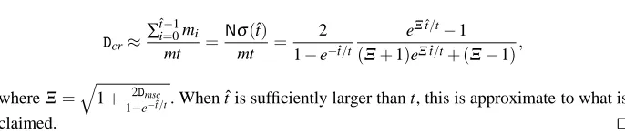
denote by ˆt, and any chain that fails to reach a DP within this bound, during either the pre-computation phase or the online phase, is discarded. The pre-pre-computation phase of a DP tradeoff must generate additional chains to fill in the discarded chains.
Even though some of our results are stated in a way that displays its dependence on ˆt, we are mainly interested in the case where ˆt is sufficiently larger than t. The number of discarded chains is minimized by such a choice and most of the pre-computation is put to good use. Since pre-computation cost is the main barrier to any large scale implementation of the tradeoff technique, such a choice is natural in practice.
If a chain is generated with the random function, the probability for it to become a DP chain within the chain length bound ˆt is
1−1−1
t
ˆt
≈1−e−ˆt/t. (9)
This easy statement may be found in [7].
2.5 Rainbow tradeoff
The rainbow table method was introduced by Oechslin [24]. From this point on, we will refer to the rainbow table method simply as the rainbow tradeoff.
2.5.1 Parameter setup
One starts with positive integers m and t satisfying the matrix stopping rule mt≈N. Notice
that this equation is different from the matrix stopping rules for the previous two algorithms. In this work, we use the notation mt=RmscNwith the matrix stopping constantRmsc=Θ(1). Unlike the previous two algorithms, a small number of tablesℓ=Θ(1)is used with the rainbow tradeoff. The parameters are always assumed to be reasonable in the sense that 1≪m,t≪N. Reduction functions Rk
j:N →N are fixed as before, but these have double
indices that are made to run over j=1, . . .,t and k=1, . . . , ℓ. The doubly colored iterating functions are defined through Fj,k=Rkj◦F.
2.5.2 Pre-computation phase
Instead of using a single reduction function for each table, t different reduction functions are sequentially applied to create a pre-computation chain of length t. Each pre-computation table stores the information from m chains. More explicitly, the i-th pre-computation chain for the k-th rainbow table takes the form
spki =xki,0
F1,k
−−−→xki,1
F2,k
−−−→xki,2
F3,k
−−−→ · · ·· · ·−−−−→Ft−1,k xk1,t−1
Ft,k
−−−→xki,t=epki,
where 1≤i≤m and 1≤k≤ℓ. Each of these is a rainbow chain.
The complete set of m chains for any fixed k is an m×t rainbow matrix and the set of pairs{(spki,epki)}iis stored as the k-th rainbow table after being sorted on the ending points.
2.5.3 Online phase
Let the inversion target y=F(x)be given for the online phase. For each j=1, . . . ,t and k=1, . . . , ℓ, we compute the j-th online chain for the k-th table
x−−−−−→Ft−j+1,k
ytk−,jj+1−−−−−→Ft−j+2,k ykt−,jj+2−−−−−→ · · ·· · ·Ft−j+3,k −−−−→Ft−1,k ykt−,j1−−−→Ft,k ytk,j,
through iterative computation, starting from the point ykt−,jj+1=Rk
t−j+1(y) =Ft−j+1,k(x).
After each chain computation, the chain end ykt,jis searched for among the ending points of
the k-th rainbow table. The absence of a collision indicates that the correct answer x does not belong to the(t−j)-th column of the rainbow matrix. The appropriate pre-computation chain is regenerated whenever a collision is found. Many of these regenerations will lead to the announcement of a false alarm.
The order of incrementing the double indices during the online phase requires clarifi-cation. One should take the chain length j-index to be the outer loop and the table number k-index to be the inner loop. In other words, for any index j, one computes the j-th online chains for allℓtables, before computing any of the(j+1)-th online chains. This is referred to as the parallel processing of rainbow tables. The opposite nesting of the loops is called the sequential processing of tables. As was already noted in [24], the parallel approach is more efficient in terms of the expected number of one-way function invocations. Parallel process-ing of tables is more commonly considered and this is the approach we assume throughout this work.
2.5.4 Success probability
In [24], one can find the success probability of a rainbow tradeoff that uses a single table written as
1−
t−1
∏
j=0
1−mNj, (10)
where m0=m and mjare recursively computed through (2). However, this was not
simpli-fied into a closed form formula there.
While studying the perfect table version of the rainbow tradeoff, the work [1] restricts to the m=Ncase and gives the approximation
t−1
∏
j=t−i
1−mNj≈t−i
t
t−i+1
t+1 . (11)
Notice that the range of indices in the left-hand side product is shorter than that appearing in (10). The left-hand side product of i terms expresses the probability for the first i on-line chain computations for a single table (non-perfect) rainbow tradeoff to fail in returning the correct answer x. This expression is valid for any m, even though the right-hand side approximation is appropriate only for m=N.
2.5.5 Preliminary analysis
A collision of points from two rainbow chains will result in merging chains only if the collision occurred at a matching color index. When a new rainbow chain is added to an existing m×t rainbow matrix that contains no collisions within each column, the probability of not experiencing a merge can be expressed as(1−m
N)t≈e−
mt
N. Hence, the matrix stopping
rule mt≈Nis the correct boundary at which collisions among pre-computation chains start
to become problematic.
Let us assume the use of a single table for the rest of this rough analysis. Ignoring collisions within each rainbow matrix column, the success probability (10) may roughly be approximated as 1− 1−m
N
t
≈1−e−mtN ≈1−1
e. This is equal to what we saw during the
rough analyses for both Hellman and DP tradeoffs.
Notice that the computations for the j-th online chain cannot reuse any of the informa-tion computed for previous online chains. Hence, the number of one-way funcinforma-tion iterainforma-tions required for the computation of all online chains is T=0+1+· · ·+ (t−1)≈t2
2. The stor-age size for the single rainbow table is M=m. Recalling the matrix stopping rule mt≈N, the tradeoff curve can be written as
T M2≈1
2
N2. (12)
The above time complexity analysis appears in [24], from which the tradeoff curve directly follows.
2.5.6 Further analysis
The preliminary analysis given above corresponds to the worst case where the complete table is processed. In practice, the online phase is likely to terminate before computing the t-th online chain. On the other hand, the cost of resolving alarms has been ignored. Hence, the rough analysis does not give the true worst case complexity.
The work [15] provides an accurate analysis of the time complexity for rainbow trade-offs. The expected number of one-way function iterations required to process a single rain-bow table was expressed as an explicit rational function ofRmsctimes t2. Similar result for the additional number of one-way function iterations required to process alarms was also stated. However, the results were restricted to the single table case. We do not state their results here, but their results are reobtained if we substituteℓ=1 into (22), appearing in the main body of this paper.
2.6 Perfect table tradeoffs
Detection of merging chains is also easily done with the rainbow tradeoff. The perfect table version of the rainbow tradeoff [24] stores information for just one chain from each set of merging chains. Unlike the DP case, a perfect rainbow matrix may contain overlapping points if they belong to different columns.
The perfect table version of the Hellman tradeoff refers to the case where the Hellman matrix contains no overlapping points. Some discussions may be found in [1, 26]. However, generating a perfect Hellman table is costly and its use is not considered to be practical.
Since there are less or no overlaps in a perfect table, these provide better coverage of the search space than their corresponding non-perfect versions for the same amount of storage. Hence, perfect tradeoffs are likely to be more efficient than the non-perfect tradeoffs. How-ever, this gain in tradeoff efficiency is paid for with the pre-computation that was wasted in generating the discarded chains.
The extra pre-computation required for the use of perfect tradeoffs may not seem to be of importance. However, the pre-computation cost can be critical when implementing trade-offs at the limit of one’s resources. Consider a large scale implementation for which the pre-computation may take several months on a large cluster of computers. In such a situa-tion, extending the pre-computation period by another few month or doubling the number of computers allocated to the pre-computation task will not be a viable option, even if it promised a significant advantage in the online tradeoff efficiency.
Even though there are analyses of perfect tradeoffs [1, 7, 8, 15, 24, 29], dealing with them at the accuracy level aimed for by the current paper is considerably more complicated than the non-perfect tradeoffs. This is especially true with the perfect DP tradeoffs. In view of relative practicality and theoretic accessibility, we deal only with the non-perfect versions of tradeoff algorithms in this work. Inclusion of the perfect tradeoffs into the comparison results obtained in this paper is left as a subject for future study.
2.7 Storage optimization
The storage size M appearing in the tradeoff curves (8) and (12) refers to the total number of starting point and ending point pairs that need to be stored in the tradeoff tables. In practice, it is important to know the physical size, or the number of bits, required for the table. Each starting point and ending point pair can surely be stored in 2 logNbits, but there
are techniques that allow more efficient use of storage.
Below, we assume a suitable method of enumerating the elements ofN has been fixed and treat elements ofN as logN-bit integers. This enumeration is trivial whenN is the set
of all bit strings of certain length, but may require a small amount of work whenN is given
as the set of passwords satisfying certain complicated linguistic structures.
2.7.1 Consecutive starting points
The first storage reduction technique we review is the use of starting points that require less storage. The work [6] does this while implementing an attack on a specific system and [7] mentions this as a well-known trick without giving any reference. A clear understanding of the random functions shows that the starting points may be chosen in any manner, as long as it has no relation to the graph structure of the specific one-way function under attack.
11101001 11001010 10111001 01101110 01011100 01010101 00101100 00010110
101001 001010 111001 101110 011100 010101 101100 010110 11
10 01 00
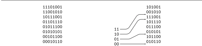
Fig. 1 Index table technique (The sorted list on the left-hand side is transformed to the right-hand side list,
which contains two less bits per entry.)
the starting points can be removed by concatenating the table index to the consecutive in-tegers [4]. Note that the table index need only be recorded once for each table. However, the effect of joining table numbers is almost nonexistent on even the second columns of the pre-computation matrices, so this detail is not very important. In any case, the starting points can be stored in log m bits, rather than logNbits.
The experiment provided by Hellman [14], supporting the arguments concerning the success probability, was executed with starting points set to small numbers, rather than ran-dom points. However, it is not clear if this was intended to reduce the storage size.
2.7.2 Taking advantage of the DP definition
In the case of DP tradeoffs, any information that can be recovered from the definition of a distinguished point may be removed from the ending point before storage. For example, if a prefix consisting of logt zero bits defines a DP, the log t bits of zeros can be removed from each ending point without any loss of information. This method was actively used in [6] and clearly stated in [29], but seems trivial enough to have been widely known before these works.
2.7.3 Index table
The work [6] introduces the index table method. This is a degenerate form of a widely known technique called hash tables, which is explained in Appendix D.
To facilitate fast table lookups, the pre-computation tables are usually sorted on the end-ing points before beend-ing written to storage. Let us focus on the{(log m)−ε}most significant bits of each ending point in the sorted table, whereεis any small positive integer. Assuming that the ending points are randomly distributed, for each integer 0≤i< m
2ε, we can expect to find approximately 2εconsecutive entries in the sorted table that have the{(log m)−ε}bit prefix of the ending point equal to integer i. Hence, one can remove{(log m)−ε}bits from each ending point and replace it with an index table that points to the starting positions for each i value without loosing any information. The number of entries contained in the index table is only2mε and hence the additional storage required by its introduction can be ignored. An example is illustrated by Figure 1.
2.7.4 Ending point truncation
The methods described so far reduce the storage size without losing any information con-cerning each starting point and ending point pair. However, this is not so with the final storage reduction method we describe, which is to simply truncate a part of the ending point before storage.
The truncation of ending points was done in [6] for a specific tradeoff implementation, where it was simply stated that the number of bits they allocate is sufficient for identification purposes. In [4]1, under the assumption that m≈N13, it is claimed that the ending points of
a DP table can be compressed to slightly more than 13logNbits. It is also claimed that the
ending points for the rainbow tradeoff can be compressed to slightly more than23logNbits.
The paper does not provide any justification for these claims.
During the online phase, when a table lookup is required, the object to be searched for in the table is truncated to the same length and compared with the truncated ending points of the table. The table lookups may now falsely return a match even when a merge between the online chain and a pre-computation chain did not happen. Still, since we were already expecting false alarms, no new measure needs to be devised to deal with the new type of false alarms. Aggressive ending point truncation will cause more frequent false alarms, hence the degree of truncation should be carefully controlled.
The word truncation may give the impression that such a method is applicable only when the spaceN consists of bit strings. On spaces that look different, any surjective map that is
pre-image uniform, in the sense that the number of pre-images for each element in the range is identical, can serve as the truncation operation. In practice, password hashes are usually bit strings and one does not apply the reduction function at the end of a chain, so truncations can easily be done.
2.8 Parameter optimization
Choosing the parameters m, t, andℓfor a concrete tradeoff implementation is not an easy task.
The work [18] starts with the assumption that the cost, in dollars, of a tradeoff attack implementation is proportional to the storage size and the number of one-way function com-putations the online phase machine can perform per unit time. This allows one to consider the lowest possible monetary cost of an attack machine that must succeed with a given probability and finish within a preset real-world time. Expressions giving lower and upper bounds for the optimal cost are presented and parameters t, m, andℓthat can achieve the optimal cost are also found. The optimal parameters that are stated depend on the relative cost of storage versus one-way function computations at unit speed.
This analysis is one of the few that takes false alarms into account when computing the time complexity of the online phase. However, the analysis relied on the bounds (5) and (6), which are not very tight, and the upper bound for the optimal cost was simply taken to be an approximation for the optimal cost. Also, while defining the optimal cost, the amount of pre-computation was fixed to what is required for a single exhaustive search.
The measure of efficiency used in the current work is different from the monetary cost discussed by [18]. Our interest is in how efficient each tradeoff algorithm is in balancing
stor-1 The paper refers to the Hellman tradeoff, but it seems that the DP tradeoff was implied. Many researchers
age against online time. This balancing ability changes with the amount of pre-computation that is invested and the required success rate. The optimal monetary cost for implementation can easily be computed whenever this balancing ability is accurately fixed.
In [17], an attempt was made to optimize the success probability of Hellman tradeoff, while keeping both the time and storage complexities constant. The gain in success proba-bility was paid for with larger pre-computation.
There are two parts of their argument that introduce inaccuracy into their results. Since they did not have access to a good expression for the time complexity, it was not possible for them to keep the time complexity exactly constant. They had to be satisfied with keeping ℓt, which is an upper bound for the time complexity in the absence of false alarms, constant. The second point was that they lacked knowledge of the exact success probability and had resorted to using its lower bound given by (5).
The general conclusions of [17] may still be correct, but the details, in particular, the explicit optimal parameters and values, will need to be recomputed with the information given in the current paper. A little more light was shed on the attempt by [24], but the discussion there still relied on rough estimates of time complexity and success probability.
2.9 Comparison of tradeoff algorithms
Let us attempt a comparison of the three tradeoff algorithms we have explained, based on their tradeoff curves that are already available. Both the Hellman and DP tradeoff curves are given by (8) and the rainbow tradeoff curve is given by (12). Considering the case where the same storage M is given to the three tradeoff algorithms, the tradeoff curves imply that the rainbow tradeoff will require only half the number of one-way function invocations compared to the other two algorithms during the online phase. In addition to giving an argument that is equivalent to what we have just describe, the work [24] argues heuristically that the rainbow tradeoff is at an advantage over the DP tradeoff concerning false alarm issues.
The claimed efficiency of the rainbow tradeoff over the DP tradeoff is refuted in [3, 4]2 with the observation that the number of physical bits required to store each entry of the tradeoff table has been ignored by [24].
Assume the use of typical parameters m=t=ℓ=N13 for the DP tradeoff. Recalling the
contents of Section 2.7, one finds that the starting points for the DP tradeoff can be stored in 13logNbits. It is claimed in [4] that the ending points can first be compressed to slightly
more than13logNbits and then further compressed to a very small number bits by applying
the index table method. Hence each entry of a DP table requires slightly more than13logN
bits to record. In the case of rainbow tradeoffs, one assumes the typical parameters m=N23,
t=N13, andℓ=1. Then each starting point requires 2
3logNbits. The ending point is first compressed to 23logNbits and then most of this is removed through the index table method.
Accepting the above arguments, we see that each entry of a rainbow table requires twice the number of bits required by an entry of a DP table. When given the same physical amount of storage, the DP tradeoff can store twice as many starting point and ending point pairs. This translates to a gain in online time by a factor of four through the tradeoff curve. In conclusion, the DP tradeoff will run two times faster than the rainbow tradeoff for the same physical amount of storage.
The more recent work [1] once again advocates the rainbow tradeoff and tries to explain that the arguments of [4] that we have explained so far are misleading. They emphasize that the advantage of the rainbow tradeoff claimed in [24] was by a factor of at least two, rather than just two. This is a reasonable point to make, but their ensuing arguments seem to indicate that they were not aware of the ending point truncation method, which was taken into account in [4]. One could interpret this as showing how uninformative [4] was in treating the ending point truncation method.
As we will verify in this work, the claims of [3, 4] were mostly correct, but there are hidden issues that can overturn their conclusion. The first is that the tradeoff curves given by (8) and (12) are not accurate. Both of these correspond to the worst case where the algorithms are executed to the end without the correct answer being found. In fact, this was the point made by [1], although it was used to support only the rainbow tradeoff. One must also note that the effects of false alarms have been ignored by both tradeoff curves so that neither accurately reflects even the worst case complexity.
The second issue is that the success probabilities of the two algorithms may not be precisely equal at the typical parameters. We have already noted that both algorithms have approximate success probability of 1−1
eat the typical parameters, but this is an extremely
rough estimate, and the running time of a tradeoff algorithm is very sensitive to the required success rate. The controversy explained here are discussed in more detail in Section 8.4, after we have developed the necessary tools.
The comparison claims by [24] and [3, 4] were made using parameters that require pre-computation equal to a single exhaustive search. Recent comparison claims that deal with the perfect tables, which we do not treat in this paper, have the tendency to completely ignore the pre-computation cost. Neither approach reflects what can be done in practice. The difficulty of including the pre-computation cost into the comparison of tradeoff algorithms seems to have been one reason why perfect tradeoffs have received more focus recently. They certainly appear more attractive, when pre-computation is ignored.
2.10 Checkpoint
The checkpoint [1] technique allows for the resolving of alarms without the regeneration of the pre-computation chain. This technique is applicable to both Hellman and rainbow tradeoffs. Application to the DP tradeoff is also possible but slightly more complicated due to the variations in chain lengths.
A column of the computation matrix is designated as the checkpoint before pre-computation. After generation of each pre-computation chain, the least significant bit of the chain element that sits at the checkpoint column is appended to the starting point and ending point pair that is to be recorded in the pre-computation table. During the online phase, we proceed as usual until an alarm is encountered. At each collision, the online chain is aligned with the colliding pre-computation chain at the ending points. If the online chain is long enough, the least significant bits of the two points that belong to the checkpoint column are compared. If the two checkpoint bits do not match, the ending point collision must have resulted from a merge of chains, and the collision is declared a false alarm. If the checkpoint bits do match, the pre-computation chain is regenerated as usual to resolve the alarm.
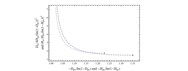
An analysis of the effects of checkpoints in reducing online time was given by [1] for the perfect rainbow tables. Analysis for Hellman tradeoffs and single table (non-perfect) rainbow tradeoffs were done in [15]. With a single checkpoint at the optimal position, the Hellman tradeoff online time decreases by 3.17% atHmsc =1, and the online time of a single table non-perfect rainbow tradeoff decreases by 5.91% atRmsc=1. The effects of checkpoints are more visible at higherHmscandRmscvalues.
The advantage of checkpoints must be compared with its side effect on the storage size. After the techniques of Section 2.7 have been applied, even a single bit difference in table entry size could translate to a meaningful size ratio change. For example, at 50 bits per table entry, if the increase of single bit per table entry caused by the use of checkpoints was instead allocated to enlarge the number of table entries, the online time would have reduced by 1− 50
51
2
=3.88%. This is better than the above mentioned 3.17% reduction effect of checkpoints on the Hellman tradeoff and the 5.91% reduction effect on rainbow tradeoff should be interpreted as achieving only approximately 2.0% extra reduction.
Since the effects of checkpoints are small and selective applications of checkpoints will affect all algorithms in the positive direction, its effect on the final comparison of algorithms will be minimal. On the other hand, consideration of the checkpoint technique would add another layer of complication to our analysis. Hence, the analysis given in the current pa-per does not consider the use checkpoints. However, we are not claiming that the use of checkpoints should not be considered in practice.
3 Applying Time Memory Tradeoff to Password Hashes
One usually states the objective of a tradeoff algorithm as the inversion of a one-way func-tion. A closer look reveals that there are two versions of the inversion problem and we will explain how one of these corresponds to the applications of the tradeoff technique to pass-word hash systems. Issues concerning the use of random functions in the theoretic analysis of tradeoff algorithms are also discussed in this section.
In this section, we refer to the one-way function image as the password hash and the input as the password.
3.1 Password hash
Let us briefly explain how the security features of many file formats that rely on passwords for access control work in its very basic form.
The designer of the system chooses and fixes a one-way function H. This one-way func-tion is a part of the file format specificafunc-tion and is usually considered to be public. In fact, the one-way function definition can be extracted from the related software even if it was not originally made public. When the owner of a file following this format wants access control to be applied to the file, the user supplies a password x. An encryption key is derived from the password, and the main content of the file is replaced by its encryption under this key. Then the image y=H(x)of the user password, under the one-way function specified for the file format, is added to the file. Finally, any record of the encryption key and the raw password supplied by the user is destroyed.
the file. If a perfect match y=H(x′)is found, equality x=x′is assumed, the main body of the file is decrypted using the key derived from the password x′, and access to the decrypted content is granted. Note that the one-way function image y of the correct password is stored within the file without any protection and is accessible to anyone that has obtained the file.
User authentication procedure for computer system logins works in much the same way. At the time of initial user registration to the system, the one-way function image of the password supplied by the user is recorded in a file that is stored within the system. In this case, access to the one-way function images may be harder for the attacker than the above case, but this information is often sent over the network in the clear to a group of computers, so that each of these computers may allow authenticated logins to a user that has registered at a central server.
3.2 Uniqueness of the pre-image to a password hash
Out of theoretic curiosity, we first ask whether a password hash uniquely determines the password. This should seem obvious in any practical usages of the password hash systems.
Proposition 1 Let H :P→H be the random function. Given any password x∈P, the
number of inputs that H maps to the password hash H(x)is expected to be 1+|P|H|−|1.
Proof Since H is the random function, we can first assign a randomly chosen value ofH
to H(x)and then define all the other function values. The probability for any one of the later assignments to strike H(x), which is an explicitly fixed value inP, is|H1|. Each later assignment is independent of all other assignments, and we can expect the number of later
assignments to H(x)to be |P|H|−|1. ⊓⊔
Readers should not misinterpret the above proposition as giving the pre-image size of a random y∈H under a random H. For the random function H, the distribution onH
produced by H(x)is the uniform distribution for each fixed x∈P, and every y∈H is
expected to have ||PH||-many pre-images, rather than 1+ |P|−1
|H| . This is not in contradiction
with the proposition, as the proposition deals with the distribution onH produced from
random inputs by the specific H that has been constructed, and this is different from the uniform distribution onH. Those points ofH that lie outside H(P), for the specifically constructed H, do not have any chance of appearing.
One can also ask for the pre-image size of a random password hash y∈H(P). Note
that this question can only be asked after the random function H has fully been constructed. The corresponding answer will depend on the size of H(P), but, when|P|=|H|, this
should be close to
|P|
E(|H(P)|)≈
1 1−1
e
≈1.582.
Once again, this question is not related to the content of the above proposition. It deals with the uniform distribution on H(P), which is different from the distribution on H(P) given by the fully specified H. Those points with larger pre-image sets will have a larger probability of appearing than those with smaller pre-image sets.
in practice, one usually assumes the use of a second ciphertext to almost uniquely identify the key. In fact, if one interprets the key to two-ciphertexts mapping as a new one-way function, then Proposition 1 claims that the key is almost uniquely determined from the two ciphertexts.
Let us next discuss what Proposition 1 implies for systems that rely on passwords for access control. These systems are usually designed so that the spaceH of potential hash values is significantly larger than the spacePof admissible passwords. A typical password hash would be a bit string of at least 128 bits in length and the number of alphanumeric passwords consisting of ten characters is only 6210≈259.5. In such a case, Proposition 1 shows that a password hash H(x), produced from a password x, will almost always identify x uniquely.
Furthermore, in practice, the set of all passwords admissible by the security system is not of much importance. Since human generated passwords are not uniformly distributed within the complete admissible password space, the tradeoff attacker first fixes a manageable sub-setP′⊂Pfrom the set of all passwords and decides to be satisfied with recovering only those passwords that lie inP′. The size of this subset is determined by the computational
power that the attacker can allocate to the pre-computation phase and should preferably cover the passwords that are most likely to be used. In fact, it has been shown [22] that human-memorable passwords can be enumerated efficiently. Under such a setting the pass-word hash setH is immensely larger than the set of passwordsP′that is being considered and hence the password hash determines the password uniquely.
For the remainder of this paper, we assume that the target system for the application of the tradeoff technique is such that|P| ≪ |H|, implying that the password hash uniquely
determines the password.
3.3 The reduction function
The tradeoff technique requires the one-way function to be iterated. Since the codomainH
of the one-way function H :P →H is usually larger than the domain P, iteration is achieved by utilizing a reduction function R :H →P. One role of the reduction function is to let a password hash be interpreted as another password. As any theoretic treatment of the tradeoff technique assumes R◦H to be a random function, let us check whether this is appropriate.
Proposition 2 Let|P|be a divisor of|H|, so that ||HP|| is an integer. Let R :H →P
be any fixed function that is pre-image uniform in the sense that it is exactly ||HP||-to-1. If H :P→H is a random function, then R◦H :P→Pis a random function.
Proof In more precise terms, we want to show that the distribution onPP, produced from the uniform distribution onHP, through the mapping H7→R◦H, is the uniform distribu-tion.
Let F0:P→P be any specific function. It suffices to show that, after random con-struction of a function H :P→H, we will find R◦H=F0with probability 1
|P||P|. Note that{R−1(z)}
z∈P is a partition ofH into cells of size | H|
|P|. The event F0=R◦H will
happen if and only if the value assigned as H(x)belongs to the cell R−1 F0(x)
, for every x∈P. Since the size of R−1 F
0(x)
independent and random for every x, the probability of arriving at F0=R◦H is
|H|/|P|
|H|
|P|
= 1
|P||P|,
as claimed. ⊓⊔
Every application of the time memory tradeoff technique to a security system involves a specific one-way function H :P→H and there is no strictly logical reason to believe that
the specific H will display the properties expected of a random function. Hence we need to discuss if predicting the behavior of an explicit tradeoff implementation with arguments concerning random functions can be justified in practice.
There can be two ways to resolve this problem. The first is to appeal to our intuition. When one ignores his knowledge of the inner working of the given specific function, it will seem as if the function is returning independently and randomly generated values to each given input. Hence, viewed from the outside, it looks as if the specific function is the random function in the construction sense. The second argument, which seems slightly more plausible, is that the one-way function used in the security system is in fact a function that has been selected from the pool of all functions. Unless we had chosen the one-way function in an unusual way, any property exhibited by a specific function will be close to the property averaged over all functions. Further discussion related to this second argument may be found in Appendix B.
We have thus partly justified the use of random functions in place of specific one-way functions H :P→H when analyzing the behavior of time memory tradeoffs. What we
have shown through Proposition 2 is that if we may treat the specific one-way function H as a random function, then the same can be done with the function R◦H :P→P. Hence,
throughout this paper, while analyzing the behavior of time memory tradeoffs, we shall work with a random function F :N →N whose domain and codomain coincide.
3.4 Two versions of the inversion problem
Discussions of this subsection should be read with the Hellman tradeoff in mind. However, the content can easily be translated to language that is appropriate for any other tradeoff algorithm.
We have already mentioned that we shall work in the situation H :P →H where
the sets satisfy|P| ≪ |H|, so that a password hash almost always determines a unique
password. We also know that any analysis of time memory tradeoff behavior is usually done with a random function F :N →N, whose image does not uniquely determine the input. In actual implementations, reduction functions Rk:H →P are defined and the online
phase algorithm works with the colored iterating functions Hk=Rk◦H :P→P.
The unique password x corresponding to inversion target y=H(x)is obtained through the tradeoff algorithm as follows. The online phase algorithm is given y and Rk(y) =Hk(x)
is passed onto its sub-algorithm that processes the k-th table. The best the sub-algorithm can do is return inputs x∈Psatisfying Hk(x) =Hk(x). Since this relation is weaker than x=x,
the parent algorithm must verify whether the password candidate x is the correct password x by testing the relation H(x) =y.