Article
Coefficient-of-determination Discrete Fourier
Transform
Matthew Marko*
1
2
3
4
5
6
NavalAirWarfareCenterAircraftDivision Joint-BaseMcGuire-Dix-Lakehurst,LakehurstNJ08733,USA1 * Correspondence:matthew.marko@navy.mil
Abstract: This algorithm is designed to perform Discrete Fourier Transforms (DFT) to convert temporaldataintospectraldata. ThisalgorithmobtainstheFourierTransformsbystudyingthe CoefficientofDeterminationofaseriesofartificialsinusoidalfunctionswiththetemporaldata,and normalizingthevariancedataintoahigh-resolutionspectralrepresentationofthetime-domaindata withafinite samplingrate. Whatisespecially beneficialaboutthisDFTalgorithmisthat itcan producespectraldataatanyuser-definedresolution.
Keywords:FourierTransform;SpectralDomain;Resolution;CoefficientofDetermination 7
1. Introduction 8
TheFourier Transform[1–7] is one of the most widely used mathematical operators in all of 9
engineering and science [8–10]. The Fourier Transform can take a temporal function and convert it into 10
a series of sinusoidal functions, offering significant clarity on the nature of the data. While the original 11
Fourier Transform is an analytical mathematical operator,Discrete Fourier Transform(DFT) methods are 12
overwhelmingly used to take incoherent temporal measurements and convert them into spectral plots 13
based on real, experimental data. 14
The author proposes a numerical algorithm to perform a highly-resolved Fourier Transform 15
of a temporal function of limited resolution. The spectral magnitude is determined by finding the 16
magnitude of the Coefficient of Determination of the function as compared with a given sinusoidal 17
function; this represents the independent spectral value as a function of the sinusoidal frequency. 18
Rather than the spectral domain being proportional to the time step, the user defines exactly which 19
frequencies are necessary to investigate. The spectral domain can be as large or as resolved as is 20
necessary; the resolution possible is limited only by the abilities of the computer performing the 21
transform. 22
2. Fourier Transform 23
The transform starts by first determining the peak total range of the data in the temporal domain, 24
this range will become the base amplitude of the spectral series. The computer then generates a series 25
of sine and cosine functions at each frequency within the spectral domain, and compares each of 26
these sinusoidal functions to the temporal data to be transformed. In the comparison, a correlation 27
coefficient is found and saved. To accommodate fluctuations in phase, each frequency generates both a 28
sine and cosine function; this ultimately results in real and imaginary spectral components. Finally, 29
1 NAVAIR Public Release 2016-755 Distribution Statement A - "Approved for public release; distribution is unlimited"
the magnitudes of the correlation factor data is normalized, and the result is an accurate spectral 30
representation of the temporal function. 31
The Fourier Transform is one of the most utilized mathematical transforms in science and 32
engineering. By definition, a Fourier Transform will take a given function and represent it by a series 33
of sinusoidal functions of varying frequencies and amplitudes. Analytically, the Fourier Transform is 34
represented as [1,2] 35
F(ω) = Z ∞
−∞f(t)·e
−2π·i·t·ωdt, (1)
whereiis the imaginary term (i=√−1),f(t)is any temporal function oftto be transformed, andω 36
(rad/s) represents the frequency of each sinusoidal function. The inverse of this function is 37
f(t) = Z ∞
−∞F(ω)·e
2π·i·t·ωdω. (2)
Conceptually, the spectral functionF(ω)represents the amplitudes of a series of sinusoidal functions 38
of frequencyω(rad/s) 39
f(t) = Σ∞n=0F(ωn)·sin(ωn·t). (3)
Often in practical application, one does not have an exact analytical function, but a series of 40
discrete data points. If it is necessary to convert this discrete data into the spectral domain, the 41
traditional approach has been to use the DFT algorithm, often known asFast Fourier Transform(FFT). 42
The DFT algorithm is, by definition [11,12] 43
Fk = ΣnN=−01xn·e
−2π·i·k·n/N. (4)
whereFkis a discrete spectral data point, andxnis a discrete data point in the temporal domain. With 44
DFT, the spectral resolution is proportional to the temporal resolution, and it is often the case that the 45
limited temporal data will not be sufficient to obtain the spectral resolution desired. 46
If one wants to obtain frequency information, there is a certain minimum temporal resolution 47
necessary to properly distinguish the frequencies; this is known as the Nyquist rate [13–17]. 48
δf = 0.5
δt (5)
As demonstrated in Table1and Figure1, two different cosine functions with frequencies of1and9 49
have exactly the same results when resolved at a temporal resolutionδt=0.1. 50
Table 1.Equal values forf=1andf=9forcos(2π·f·x).
x f=1 f=9
There are many approaches to implementing Fourier transforms on data of limited resolution. 51
One method is to introduce a scaled coordinate system and identifying the Fourier variables as the 52
direction cosines of propagating light have been used to spectrally characterize diffracted waves in 53
a method known as Angular Spectrum Fourier transform (FFT-AS) [18–21]. Another technique of 54
numerical Fourier Transform is Direct Integration (FFT-DI) [22], using Simpson’s rule to improve the 55
calculations accuracy. Finally, one of the simplest approaches to taking the Fourier transform with a 56
limited temporal resolution is to use Non-uniform Discrete Fourier Transforms (NDFT) [23–31] 57
Fk = ΣNn=−01xn·e−2π·i·pn·ωk. (6)
where 0<pn <1 are relative sample points over the range, andωkis the frequency of interest. 58
3. Algorithm 59
This algorithm, which the author calls theCoefficient of Determination Fourier Transform(CDFT), is 60
an approach to obtain greater spectral resolution; the full spectral domain, or any frequency range or 61
resolution desired, is determined by the user. Greater resolution or a larger domain will inherently 62
take longer to solve, depending on the computer resources available. One advantage of this approach 63
is that the spectral domain can also have varying resolutions, for enhanced resolution at points of 64
interest without dramatically increasing the computation cost of each Fourier Transform. 65
At each discrete point in the spectral domain, the algorithm generates two sinusoidal functions 66
Fn(t) = A·cos(2π·ωn·t), (7)
ˆ
Fn(t) = A·sin(2π·ωn·t),
whereFn(t)is to represent the real spectral components, ˆFn(t)is to represent the imaginary spectral 67
components,ωnis the discrete frequency of interest,tis the independent variable of the data of interest, 68
andAis the amplitude of the function, 69
A = max{f(t)} −min{f(t)}, (8) defined and the total range within the temporal data.
70
The next step is to take each of these functions, and find theCoefficient of Determination(CoD) 71
between the function and the temporal data, all with the same temporal domain and resolution 72
[9,32–35]. The CoD is a numerical representation of how much variance can be expected between 73
two functions. To find the CoD between two equal-length discrete functionsFn(t)and fn(t), three 74
coefficients are first calculated 75
SSt = ΣNn=1(Fn(t)−F¯n)·(fn(t)−f¯n),
SS1 = ΣNn=1(Fn(t)−F¯n)2, SS2 = ΣNn=1(fn(t)−f¯n)2,
whereNis the discrete length of the two functions, and ¯Fnand ¯fnrepresent the arithmatic mean value 76
of functionsFnand fn. The CoD, represented asR, is then determined as 77
R = √ SSt SS1·SS2
and the closer the two functions match, the closer the value of the CoD reaches 1. If there is no match at 78
all, the CoD will be equal to 0, and if the two functions are perfectly opposite of each other (Fn=−fn), 79
the CoD goes up to -1. In practice, the CoD is often represented as theR2value, 80
R2 = SS
2 t
SS1·SS2. (10)
This process is repeated for every sine and cosine function generated with each frequency within the 81
spectral domain. The coefficients of determinations can be used to represent the spectral values, both 82
real (cosine function) and imaginary (sine functions), for the given discrete frequency point. These 83
functions ofRvalues for the real and imaginary components are then normalized to the maximum 84
real and imaginary values, and multiplied by the amplitudeAdetermined in equation8. The final 85
outcome is a phase-resolved spectral transformation of the input function, but with a spectral domain 86
as large or resolved as desired. 87
Finally, this spectral transformation can easily be converted back to the temporal domain. By 88
definition, the temporal domain is merely the sum of the series of sinusoidal waves, and thus the 89
inverse Fourier transform can simply be defined as 90
f(t) = ΣNm=1{real(Fm)·cos(ωm·t)}+{imag(Fm)·sin(ωm·t)}. (11) 4. Initial Demonstration of Algorithm
91
To demonstrate the capability of this algorithm, six functions are generated based on the two 92
similar functions demonstrated in Table1and Figure1; the two functions are used with a temporal 93
range of 0 to 1, with the same temporal resolution ofδt=0.1, and frequencies of bothf=1andf=9. The 94
cosine functions are modified to have a phase shift of±2π/3. 95
The Fourier transform was taken of all six of these functions with both the CDFT algorithm, as 96
well as the NDFT algorithm defined in equation6. The spectral magnitude and phase from both 97
methods are plotted in Figure2. By using equation11to get back to the temporal domain, all six 98
functions matched with the spectral magnitude and phase from the CDFT; there is no coherent match 99
for the NDFT. This is realized by finding the coefficient of determination between the recovered 100
temporal data and the original temporal data; theR2results are tabulated in Table2. While the NDFT 101
may give a clear picture of the spectral domain of the function, it is impossible to recover the function 102
back to the original temporal domain without excessively computationally intensive matrix analysis. 103
The strength of CDFT transform lies in its inverse operator defined in equation11, with which the true 104
temporal function can be obtained back from the spectral domain obtained with highly resolved CDFT. 105
Table 2. Correlation between the original temporal function and the temporal function retrieved (equation11) from the spectral plot obtain with both CDFT and NDFT (Figures2).
f (Hz) Phase R2CDFT R2NDFT
1 0 0.9999 0.1197
1 2·π/3 0.9967 0.0091 1 -2·π/3 0.9964 0.0163
9 0 0.9999 0.1197
9 2·π/3 0.9964 0.0163 9 -2·π/3 0.9967 0.0091
5. Parametric Study 106
A parametric study of this transform was conducted, to demonstrate that it can be used for high 107
resolution measurements of the spectral frequency with a limited temporal resolution. To demonstrate 108
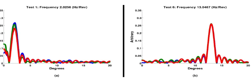
Figure 4.Spectral results of the randomly generated functions, for frequencies of (a) 2.0256 (Hz/Rev) and (b) 13.0467 (Hz/Rev), but for different phases, magnitudes, and random noises.
measured window. Both the independent and dependent temporal variables are arbitrary values to 110
demonstrate the transform function; the independent scale ranges from 0 to 1 and has 180 data points. 111
The arbitrary dependent data had random averages between -1000 and 1000, with an amplitude of 112
200 and random noise to represent the typical randomness found in typical test data. Each of these 15 113
random frequencies was phase shifted by three random phases. All forty-five arbitrary functions were 114
transformed into the spectral domain with this transform, with a frequency domain ranging from 0 to 115
20 cycles per unit time duration, and a frequency resolution of 1 mHz; two examples of these spectral 116
results are presented in Figure4. As a further test of the robustness of the transform, the spectral data 117
was then converted back to the temporal domain, and the new temporal function was compared to the 118
original function with the coefficient of determination method to ascertain errors from the transform. 119
This Fourier transform was remarkably effective at finding the peak primary frequency, often 120
with accuracy’s down to tens of mHz. The functions of the peak frequencies (Figure5), both which 121
were used for the initial function and the peak of the Fourier transform, matches with anR2value 122
of 0.999991; effectively identical. The functions of the random phase angle at the peak frequencies 123
(Figure6), both which were used for the initial function and the phase of the Fourier transform at the 124
peak frequency, matches with anR2value of 0.9982; demonstrating that this transform can be used to 125
capture both spectral magnitude and phase with great accuracy. 126
Finally, the inverse of this Fourier transform was conducted for each spectral output, and the 127
errors between the original functions and the transformed-inverse-transformed function are minimal. 128
As expected, not all of the fine random noise is captured; this would require a near infinite spectral 129
domain, which would further increase computational costs, but the overarching shapes, magnitudes, 130
and phases of the functions are consistently captured. Taking the coefficient of determination squared 131
of each function pair, the value ofR2is never less than 0.92. Two examples of the original function 132
(lines) and the transformed-inverse-transformed function (stars) are represented in Figure7. The 133
tabulated results of all fifteen studies, for each of the three phase magnitude shifts, are demonstrated 134
in Tables3-5. 135
6. Conclusion 136
This effort has demonstrated a practical, working, invertible method of numerically conducting a 137
Fourier Transform, obtaining high-resolution in the spectral domain from limited resolution in the 138
temporal domain, and retaining the ability to go back to the temporal domain from the spectral data 139
with equation11. While the CDFT transform inherently is more computationally expensive than 140
traditional DFT and NDFT methods, any desired spectral resolution and spectral domain can be used 141
to characterize the input data; the transform can even convert the function to a spectral domain of 142
varying resolution, so that peaks can be accurately identified without too much computational expense. 143
The algorithm was tested at fifteen different random frequencies, all with three different random 144
Figure 6.Angle Prediction Results,R2=0.9982
Table 3.Comparison of Results, for Phase Shift Angle 1.
Test Max Freq Max Freq sin(Phase) sin(Phase) R2 Original CFT Result Original CFT Result (Temporal) 1 2.0256 2.095 -0.72837 -0.56129 0.92791 2 10.6771 10.678 0.88707 0.88349 0.94843
3 5.5118 5.537 0.82648 0.76277 0.94092
4 11.1441 11.146 0.32585 0.30499 0.93117
5 4.1527 4.137 0.020562 0.14696 0.93132
6 13.0467 13.05 0.94015 0.94829 0.93359
7 11.9742 11.973 -0.31888 -0.32338 0.92769 8 11.3472 11.339 0.78318 0.78725 0.93398 9 12.5892 12.578 -0.35645 -0.31945 0.93956
10 11.128 11.122 0.90871 0.90812 0.92836
11 3.9531 3.954 -0.20131 -0.20166 0.93636
12 5.6981 5.677 0.080619 0.14678 0.93363
13 16.1721 16.158 0.38625 0.41684 0.94243
14 12.2989 12.32 0.57446 0.63023 0.93483
15 10.0715 10.085 -0.43758 -0.3967 0.92398
Table 4.Comparison of Results, for Phase Shift Angle 2.
Test Max Freq Max Freq sin(Phase) sin(Phase) R2 Original CFT Result Original CFT Result (Temporal) 1 2.0256 2.026 -0.062681 -0.056313 0.93311 2 10.6771 10.658 0.25575 0.18466 0.93944
3 5.5118 5.511 0.54959 0.54223 0.9434
4 11.1441 11.166 -0.90216 -0.87023 0.93194 5 4.1527 4.141 -0.92686 -0.92268 0.92885 6 13.0467 13.031 -0.64986 -0.6287 0.92476 7 11.9742 11.97 -0.95715 -0.95146 0.93294 8 11.3472 11.344 0.16368 0.17658 0.92725 9 12.5892 12.593 -0.25732 -0.23808 0.94473
10 11.128 11.145 0.86293 0.90011 0.93841
11 3.9531 3.97 0.65591 0.69795 0.94498
12 5.6981 5.7 -0.62372 -0.63233 0.93151
13 16.1721 16.169 0.76013 0.75789 0.93039
14 12.2989 12.31 -0.99804 -1 0.93751
15 10.0715 10.084 0.9865 0.98098 0.9411
peak frequency and phase angle remarkably, with a higher degree of accuracy than one can expect 146
with traditional DFT methods. 147
Supplementary Materials:The following are available online, Run_Initial_Study.zip 148
Acknowledgments: The author would like to acknowledge Lou Vocaturo and Kevin Larkins for useful 149
discussions. 150
Author Contributions:M.M. is the sole author of this manuscript. 151
Conflicts of Interest:The founding sponsors had no role in the design of the study; in the collection, analyses, or 152
interpretation of data; in the writing of the manuscript, and in the decision to publish the results. 153
Abbreviations 154
The following abbreviations are used in this manuscript: 155
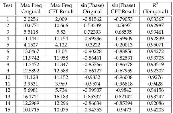
Table 5.Comparison of Results, for Phase Shift Angle 3.
Test Max Freq Max Freq sin(Phase) sin(Phase) R2 Original CFT Result Original CFT Result (Temporal) 1 2.0256 2.009 -0.81562 -0.79053 0.93367
2 10.6771 10.666 0.58339 0.5697 0.92987
3 5.5118 5.53 0.72393 0.68535 0.93461
4 11.1441 11.154 -0.99286 -0.99909 0.92839
5 4.1527 4.122 -0.3222 -0.20013 0.95071
6 13.0467 13.04 -0.90228 -0.88856 0.94272 7 11.9742 11.958 -0.86461 -0.82531 0.93705 8 11.3472 11.347 -0.85766 -0.86378 0.93519 9 12.5892 12.588 -0.66127 -0.67959 0.92307 10 11.128 11.152 -0.9832 -0.96008 0.9276
11 3.9531 3.969 -0.9574 -0.96818 0.9428
12 5.6981 5.734 -0.99907 -0.9842 0.94156
13 16.1721 16.183 0.85337 0.82142 0.93247 14 12.2989 12.296 -0.86634 -0.85394 0.92086 15 10.0715 10.075 -0.94753 -0.9473 0.94203
MDPI Multidisciplinary Digital Publishing Institute DOAJ Directory of open access journals
DFT Discrete Fourier Transform FFT Fast Fourier Transform
NDFT Non-uniform Discrete Fourier Transform
CDFT Coefficient of determination Discrete Fourier Transform CoD Coefficient of Determination
157
Bibliography 158
1. Nagel, R.K.; Saff, E.B.; Snider, A.D. Fundamentals of Differential Equations, 5thEdition; Addison Wesley: 75 159
Arlington Street, Suite 300 Boston, MA 02116, 1999. 160
2. Haberman, R.Applied Partial Differential Equations With Fourier Series and Boundary Value Problems, 4thEdition; 161
Prentice Hall: Upper Saddle River, New Jersey, 2003. 162
3. Harris, F.J. On the Use of Windows for Harmonic Analysis with the Discrete Fourier Transform. Proceedings 163
of the IEEEJanuary 1978,66, 51–83. 164
4. Dorrer, C.; Belabas, N.; Likforman, J.P.; Joffre, M. Spectral resolution and sampling issues in Fourier-transform 165
spectral interferometry. Journal of Optics Society of America B2000,17, 1795–1802. 166
5. Arfken, G.B.; Weber, H.J.Mathematical Methods for Physicists, Sixth Edition; Elsevier: 30 Corporate Drive, Suite 167
400, Burlington MA 01803, 2005. 168
6. Zill, D.G.; Cullen, M.R. Advanced Engineering Mathematics, Second Edition; Jones and Bartlett Publishers: 169
Sudbury MA, 2000. 170
7. Numerical Recipies in C: The Art of Scientific Computing; Cambridge University Press, 1988; chapter 13, pp. 171
584–591. ISBN 0-521-4310805. 172
8. Chen, W.H.; Smith, C.H.; Fralick, S.C. A Fast Computational Algorithm for the Discrete Cosine Transform. 173
IEEE Transactions on CommunicationsSeptember 1977,25, 1004–1009. 174
9. Agarwal, R.C. A New Least-Squares Refinement Technique Based on the Fast Fourier Transform Algorithm. 175
Acta Cryst.1978,34, 791–809. 176
10. Finzel, B. Incorporation of fast Fourier transforms to speed restrained least-squares refinement of protein 177
structures. Journal of Applied Cryst.1986,20, 53–55. 178
11. Garcia, A. Numerical Methods for Physics, Second Edition; Addison-Wesley: 75 Arlington Street, Suite 300 179
Boston, MA, 1999. 180
12. Poon, T.C.; Kim, T.Engineering Optics With Matlab; World Scientific Publishing Co: 27 Warren St, Hackensack, 181
13. Nyquist, H. Certain Topics in Telegraph Transmission Theory.Proceedings of the IEEE2002,90, 280–305. 183
14. Landau, H.J. Necessary Density Conditions for Sampling and Interpolation of Certain Entire Functions. 184
Acta Mathematica1967,117, 37–52. 185
15. Shannon, C.E. Communication in the Presence of Noise. Proceedings of the IEEE447-457,86, 1998. 186
16. Luke, H.D. The Origins of the Sampling Theorem. IEEE Communications Magazine1999,April, 106–108. 187
17. Kupfmuller, K. On the Dynamics of Automatic Gain Controllers. Elektrische Nachrichtentechnik2005, 188
5, 459–467. 189
18. Harvey, J. Fourier treatment of near-field scalar diffraction theory. American Journal of Physics1979, 190
47, 974–980. 191
19. Jiang, D.; Stamnes, J.J. Numerical and experimental results for focusing of two-dimensional electromagnetic 192
waves into uniaxial crystals.Optics Communications2000,174, 321–334. 193
20. Stamnes, J.J.; Jiang, D. Focusing of electromagnetic waves into a uniaxial crystal. Optics Communications 194
1998,150, 251–262. 195
21. Jiang, D.; Stamnes, J.J. Numerical and asymptotic results for focusing of two-dimensional waves in uniaxial 196
crystals.Optics Communications1999,163, 55–71. 197
22. Shen, F.; Wang, A. Fast-Fourier-transform based numerical integration method for the Rayleigh–Sommerfeld 198
diffraction formula. Applied Optics2006,45, 1102–1110. 199
23. Boyd, J.P. A Fast Algorithm for Chebyshev, Fourier, and Sine Interpolation onto an Irregular Grid.Journal of 200
Computational Physics1992,103, 243–257. 201
24. Lee, J.Y.; Greengard, L. The type 3 nonuniform FFT and its applications. Journal of Computational Physics 202
2005,206, 1–5. 203
25. Dutt, A. Fast Fourier Transforms for Nonequispaced Data. PhD thesis, Yale University, 1993. 204
26. Dutt, A.; Rokhlin, V. Fast Fourier Transforms for Nonequispaced Data II.SIAM Journal of Scientific Ccomputing 205
1993,14, 1368–1393. 206
27. Dutt, A.; Rokhlin, V. Fast Fourier Transforms for Nonequispaced Data II.Applied and Computational Harmonic 207
Analysis1995,2, 85–100. 208
28. Greengard, L.; Lee, J.Y. Accelerating the Nonuniform Fast Fourier Transform. SIAM Review2004,46, 443–454. 209
29. Dohler, M.; Kunis, S.; Potts, D. Nonequispaced Hyperbolic Cross Fast Fourier Transform. SIAM Journal on 210
Numerical Analysis2010,47, 4415–4428. 211
30. Fessler, J.A.; Sutton, B.P. Nonuniform Fast Fourier Transforms Using Min-Max Interpolation. IEEE 212
Transactions on Signal Processing2003,51, 560–574. 213
31. Ruiz-Antolin, D.; Townsend, A. A Nonuniform Fast Fourier Transform Based on Low Rank Approximation. 214
SIAM Journal on Scientific Computing2018,40, 529–547. 215
32. Cameron, A.C.; Windmeijer, F.A. An R-squared measure of goodness of fit for some common nonlinear 216
regression models. Journal of Econometrics1997,77, 329–342. 217
33. Magee, L. R2 Measures Based on Wald and Likelihood Ratio Joint Significance Tests.The American Statistician 218
August 1990,44, 250–253. 219
34. Nagelkerke, N.J.D. A note on a general definition of the coefficient of determination. Biomelrika1991, 220
78, 691–692. 221
35. Strang, G.Introduction to Linear Algebra, 3rdEdition; Wellesley-Cambridge Press: 7 Southgate Rd, Wellesley, 222