Article
Four Particular Cases of the Fourier Transform
Jens V. Fischer
GermanAerospaceCenter(DLR),MicrowavesandRadarInstitute,82234Wessling,Germany; jens.fischer@dlr.de,Tel.:+49-8153-28-3057
Abstract: Inprevious studieswe used Laurent Schwartz’ theoryof distributions to rigorously introduce discretizations and periodizations on tempered distributions. These results are now usedinthisstudytoderiveavaliditystatementforfourinterlinkingformulas. Theyarevariantsof Poisson’sSummationFormulaandconnectfourcommonlydefinedFouriertransformstooneanother, theintegralFouriertransform,theDiscrete-TimeFourierTransform(DTFT),theDiscreteFourier Transform(DFT)andtheIntegralFouriertransformforperiodicfunctions–usedtoanalyzeFourier series.Weprovethatundercertainconditions,thesefourFouriertransformsbecomeparticularcases oftheFouriertransforminthetempereddistributionssense.Wefirstderivefourinterlinkingformulas fromfourdefinitionsoftheFouriertransformpuresymbolically.Then,usingourpreviousresults, wespecifythreeconditionsforthevalidityoftheseformulasinthetempereddistributionssense.
Keywords: Fourier transform; Fourier series; DTFT; DFT; generalized functions; tempered distributions;Schwartzfunctions;PoissonSummationFormula;discretization;periodization
MSC:42B05,42B08,42B10,46F05,46F10
1. Introduction
Poisson’s Summation Formula plays a very central role in mathematics. Its generalization tells us that discretizations and periodizations are dual operations and due to their reciprocity one of the two sums converges faster than the other. It can e.g. be used to speed up summations [1]. In this study, we will see that there are basically two variants of these formulas. We refer to the ones given in Gasquet [2], equations (37.1) and (37.2), as
+∞
∑
k=−∞f(t−kT) = 1 T
+∞
∑
k=−∞ˆ
f(k T)e
2πtTk (1)
and
+∞
∑
k=−∞ˆ
g(σ− k
T) =T +∞
∑
k=−∞g(kT)e−2π σkT (2)
whereT>0 is real and ˆf and ˆgdenote the Fourier transforms of f andg, respectively. As can easily be seen, these two reduce to special variants of the Poisson Summation Formula ift=0 orσ=0 or ifT= 1. Choosingt=0 andT= 2πin (1), yields the formula originally found by Poisson [1,3–6]. Another variant arises if f is the Dirac impulseδ, i.e., a tempered distribution [5], or ifgis the function that is constantly 1, i.e., a non-integrable function. Choosing, vice versa,g=δorf =1, both equations fail. Equivalently, if one choosesg = sincand f = rect, letsinc(t) := sin(πt)/(πt)andrectbe its Fourier transform, they hold. But choosing f =sincorg =rect, they fail. In this paper, we use two
simple criterions found in a previous study [6], which are dual to one another, for deciding whether a Poisson Summation Formula of type (1) or (2) will hold or fail in the tempered distributions sense. Our results will then be used in order to decide under what conditions four usually defined Fourier transforms (Section7.1) will hold in the tempered distributions sense and reduce to only one Fourier transform, the Fourier transform on tempered distributions (Section7.2).
Section2prepares the reader to the particularities of the space of tempered distributions. Readers who are familiar with Laurent Schwartz’ theory of distributions may skip this section. Section3
introduces to the notations and the terminology used and Section4prepares the theorem given in Section5. In Section6, we discuss these findings.
2. Preliminaries
2.1. The Fourier Transform and the Theory of Infinitely Differentiable Functions
Whenever we use the Fourier transform, we actually develop a functionf, no matter whether it is differentiable or not, into a superposition (integral)
f(t) = Z ∞
−∞c(σ)e 2πitσdσ
of infinitely differentiable functionse2πitσ where c(σ) are the coefficients. Hence, functions that
can be Fourier transformed must unconditionally be infinitely differentiable in some sense. The theory that made this notion rigorous is the theory of distributions (generalized functions theory) summarized in Laurent Schwartz’ encompassing two-volume work [7–9]. It has already become a standard setting in Fourier analysis [2,5,10–15], wavelet theory [16] and beside mathematics [17–30], also in quantum physics [31–34] where its origin [35], the Dirac delta [36] can be found, and in electrical engineering [37,38] where the Dirac delta is used to formally describe sampling [39]. Laurent Schwartz’ theory of distributions is also part of wider theories, such as those on pseudo-differential operators [40–42] or modulation spaces [43–45] including Feichtinger’s algebra [46]. Compared to these wider theories, the approach in this study requires less precautions. We only rely on three subspaces of the space of tempered distributions in Laurent Schwartz’ standard distribution theory [9,21–25]. All functions and generalized functions will be kept infinitely differentiable in this way.
The circumstance that convolutions and, correspondingly, multiplications among distributions cannot arbitrarily be applied, is sometimes considered a major disadvantage of Laurent Schwartz’ distribution theory [47,48]. It is, however, not a disadvantage of the theory – it is rather owned to Heisenberg’s uncertainty principle [30]. Intuitively it is clear that convolutions fail if they are not summable. Equivalently, the corresponding multiplications must fail because they are coupled via the Fourier transform. Any other outcome would violate the fact that multiplications and convolutions correspond to one another in dual domains. So, when convolutions fail, their corresponding multiplications fail and, vice versa, when multiplications fail, their corresponding convolutions fail. We therefore stay, for convenience only, within the space of tempered distributionsS0where we have a clear understanding of the Fourier transform as an automorphism on tempered distributions, where we will be able to infinitely derive all functions and where we have a clear understanding of allowed multiplications and convolutions among distributions. They are regulated in Laurent Schwartz’ theorem on the multiplication-convolution equivalence inS0, presented as Lemma1in the next section – for the readers convenience. Another consequence of this central law is the circumstance that discretizations and periodizations on tempered distributions cannot arbitrarily be allowed. One may recall that discretization, in other words, "sampling" of a generalized function can be defined by
multiplyingit with a Dirac comb [1,10,49]
IIIT(t):= +∞
∑
k=−∞3 of 19
whereT > 0 is real-valued andδkT := τkTδextends toτkTf := f(t−kT)for ordinary functions f.
Let us write III instead of IIIT ifT = 1. Equivalently, the periodization of a generalized function
can be defined byconvolvingit with a suitable Dirac comb [1,10,49]. Therefore, in a most rigorous approach, these operations must obey Laurent Schwartz’ equivalence of allowed multiplications and convolutions within the space of tempered distributions.
2.2. Convolution vs. Multiplication
Because of the fact that both, convolution and multiplication, may fail among arbitrary tempered distributions, we need to consider three important subspaces of the spaceS0of tempered distributions. For a deeper understanding one may refer to [6,19–25,29,30,50–55]. We require the subspaceOC0of
convolution operators inS0, the subspaceOM of multiplication operators inS0 and the Schwartz
space S which consists of (ordinary) functions which are both, convolution and multiplication operators. All three were introduced by Larent Schwartz [9]. We build on the following theorem which can also be found in Trèves [20], Horváth [21] and Barros-Neto [24] for the reader’s convenience. It plays a very central role in Laurent Schwartz’ theory of distributions because it extends the commonly known duality between multiplication and convolution to the space of tempered distributions.
Lemma 1(Convolution vs. Multiplication). Let g∈ S0, f ∈ OC0andα∈ O
M, then
F(g∗f) =F(g)· F(f) and (3)
F(g·α) =F(g)∗ F(α) (4)
hold in the tempered distributions sense. 2.3. Discretization vs. Periodization
Using Lemma1and the fact that III ∈ S0 andF(III) = III, see e.g. [5], one easily verifies the following lemma where we may think of "III∗f" as the periodization of f with increments ofT=1 and of "III·α" as the discretization ofαat integers.
Lemma 2(Discretization vs. Periodization). Let f ∈ OC0andα∈ OM, then
F(III∗f) =F(III)· F(f) and (5)
F(III·α) =F(III)∗ F(α) (6)
hold in the tempered distributions sense.
The role of III as an ideal sampling and periodization operator can be studied in Kammler [10] or Bracewell [49], for example. Hence, by using444f := III∗ f and⊥⊥⊥α := III·α, where 444is periodization and⊥⊥⊥is discretization (sampling), the latter lemma becomes
F(444f) =⊥⊥⊥(Ff) and (7)
F(⊥⊥⊥α) =444(Fα) (8)
in the tempered distributions sense. It tells us that "periodizing f discretizes its Fourier transform" and, vice versa, "discretizingαperiodizes its Fourier transform". Without loss of generality, one may think ofαas the Fourier transform Ff =α of f. Allowing moreover arbitrary incrementsT>0, i.e., using the definition444Tf :=IIIT∗f and⊥⊥⊥Tα:=IIIT·αwe obtain
F(444Tf) = 1
T ⊥⊥⊥1T(Ff) and (9)
F(⊥⊥⊥1
in the tempered distributions sense [29], due to the reciprocity between time and frequency domain. However, it is worth noting that the opposite, i.e., "discretizing f" and "periodizingα" is not allowed most arbitrarily. It requires thatα,f ∈ OM∩ OC0, as described below.
2.4. Poisson’s Summation Formula
One may think of the formulas (5), (6) and (7), (8) as well as (9), (10) as generalized versions of the Poisson Summation Formula and its dual [2,4]. This can be seen by inserting the definition of444Tand applying the Fourier transform ruleF−1{
δ(σ−Tk)}=e2πt
k
T in (1). It becomes
(444Tf)(t) = 1 T F
−1{ +
∑
∞ k=−∞ˆ
f(k T)δ(σ−
k
T)} (11)
and inserting the definition of⊥⊥⊥1
T on the right and applyingF on both sides, it yields (9).
Vice versa, inserting the definition of 4441
T and applying the Fourier transform rule
F {δ(t−kT)}=e−2π σkTin (2) yields
(4441
Tg)(t) =ˆ TF { +∞
∑
k=−∞g(kT)δ(t−kT)} (12)
and inserting the definition of⊥⊥⊥Ton the right and dividing both sides byT, it yields (10).
Let us recall now that (3), (5), (7), (9), (11) and (1) are true if f ∈ OC0 and (4), (6), (8), (10), (12)
and (2) are true ifα ∈ OMaccording to Lemma1and Lemma2. BecauseFf = α, it is moreover sufficient to either fulfillf ∈ OC0orα∈ OMasF(OC0) =OMandF(OM) =OC0, see e.g. [9,20,21].
These two conditions form, accordingly, an outer framework for validity statements on variants of the Poisson Summation Formula in the tempered distributions sense. They in particular apply to (1) and (2) and therewith to many variants of the Poisson Summation Formula found in the literature.
2.5. Validity Statement
The validity statement f ∈ OC0 and, equivalently, α ∈ OM is moreover most general inS0
because it cannot be widened up in any way. The space OC0 already includes all convolution
operators andOM already includes all multiplication operators and beyond these two spaces no
other convolution or multiplication will be possible inS0. It is clear that otherwise the corresponding generalized function already belongs to one of these two spaces. This validity statement is furthermore obtained in good agreement with many other publications devoted to this topic, including [4,56–60], except for the fact that, in this as well as in our previous studies, we generally do not move away from the overall principle that all functions must be infinitely differentiable. It is the default, tacit assumption in distribution theory.
One now easily verifies that in order to sample a tempered distributionf, it must be smooth in the ordinary functions sense and should not grow faster than any polynomial. If one of these two conditions is not fulfilled, then f is either no tempered distribution or f is not bandlimited. If f is not bandlimited (in the sense thatFf ∈ OC0) then its Fourier transformFf cannot be periodized, i.e., the
5 of 19
Table 1.Discrete Functions vs. Periodic Functions
No Rule Remark Requirement
1 F(444Tf) = 1 T ⊥⊥⊥1
T(Ff) Poisson Summation Formula (generalized) f ∈ OC 0, T>0
2 F(⊥⊥⊥1
Tf) = T444T(Ff) Poisson Summation Formula (its dual) f ∈ OM, T>0 3 F(444f) = ⊥⊥⊥(Ff) Rule 1, special caseT=1 f∈ OC0
4 F(⊥⊥⊥f) = 444(Ff) Rule 2, special caseT=1 f ∈ OM
5 F(444δ) = ⊥⊥⊥(Fδ) Rule 3, special casef ≡δandFδ=1 –
6 F(⊥⊥⊥1) = 444(F1) Rule 4, special casef ≡1 andF1=δ –
7 F(444δ) = 444δ Rule 5 + 9, Dirac Comb Invariance –
8 F(⊥⊥⊥1) = ⊥⊥⊥1 Rule 6 + 9, Dirac Comb Invariance –
9 444δ = ⊥⊥⊥1 Dirac Comb Identity (by definition) –
10 ⊥⊥⊥T1 = 444Tδ Dirac Comb Identity (by definition) T>0
11 F(444Tδ) = 1T ⊥⊥⊥1
T1 Rule 1, f≡δ, Dirac comb reciprocity T>0 12 F(⊥⊥⊥1
T1) = T444Tδ Rule 2, f≡1, Dirac comb reciprocity T>0 13 F(f∗g) = Ff· Fg Convolution vs. Multiplication f∈ OC0
14 F(f·g) = Ff∗ Fg Multiplication vs. Convolution f ∈ OM
15 444g∗ f =444(g∗f) =g∗ 444f Periodization Rule f,g∈ OC0
16 ⊥⊥⊥g· f =⊥⊥⊥(g·f) =g·⊥⊥⊥f Discretization Rule f,g∈ OM
17 444δ∗ f =444(δ∗f) =444f Rule 15,g≡δ, Periodization off f∈ OC0
18 ⊥⊥⊥1· f =⊥⊥⊥(1·f) =⊥⊥⊥f Rule 16,g≡1, Discretization of f f ∈ OM
19 444(rect) =1 Rule 17,f ≡rect, Periodization ofrect –
20 ⊥⊥⊥(sinc) =δ Rule 18,f ≡sinc, Discretization ofsinc –
3. Notation
3.1. Generalized Functions
Although generalized functions cannot be treated pointwise and must always be applied as a whole, we nevertheless denote them as f(t)instead of f to indicate that they would depend ont∈Rn
orσ ∈ Rn or k ∈ Zn or m ∈ Zn if they were ordinary functions. We denote Fourier transformed
functions as(Ff)(σ) = fˆ(σ)orF(f) = fˆor justFf and we denote discrete functions as f[k]or ˆf[m], respectively. For simplicity, we do not assume vector-valued functions in this study, i.e., we letn=1 int,σ∈Rnork,m∈Znalthough the n-dimensional case looks very similar. For cases ofn>1, one
may refer to our previous studies [6,29,30].
3.2. Definitions
As explained above, discretizations and periodizations, may fail on tempered distributions. In order to avoid this and to make our definitions rigorous, we require according to Lemma2, that only
f ∈ OMcan be discretized and onlyf ∈ OC0 can be periodized. For any f ∈ OM, any real-valued T>0,k∈Zand the Dirac comb III∈ S0, one may therefore define
(⊥⊥⊥Tf)(t) := (IIIT·f)(t) = ∞
∑
k=−∞and for any f ∈ OC0one may define
(444Tf)(t) := (IIIT∗f)(t) = ∞
∑
k=−∞f(t−kT) (14)
where (13) is called the "discretization of f" and (14) is called the "periodization of f" with incrementsT. The result⊥⊥⊥Tf of discretization is again a tempered distribution. Equivalently, the result444Tf of
periodization is again a tempered distribution. We call⊥⊥⊥Tf "discrete function" and444Tf "periodic function". It is either a periodic function in the usual sense or a generalized periodic function, such as the Dirac comb IIITwhich is T-periodic. Vice versa, every ordinary or generalized T-periodic function gcan be written asg = 444Tf for some f ∈ OC0. Equivalently, for every discrete functiong= ⊥⊥⊥α there is someα∈ OM. It is interesting to note in this context that both these operations have already
been defined in 1953 in Woodward [1] and later in Brandwood [14] with symbolscombandrepinstead of⊥⊥⊥and444, but pure symbolically, i.e., without statement on the actually permitted domain and the
resulting image of these operations in the tempered distributions sense.
4. Calculation Rules
4.1. Schwartz Functions
We first need to have a closer look at functions which are ordinarily smooth together with their Fourier transform. It is expressed in the conditionϕ∈ OM∩ OC0. The spaceOMcontains all ordinarily
smooth tempered distributions andOC0=F(OM)contains all those tempered distributions whose
Fourier transform is ordinarily smooth. One may recall thatF(OC0) =OM. Let us call them "fully
smooth functions". A trivial statement is the following. It merely results from the usual staggered, continuous embeddings of subspaces [9,29,54] within the space of tempered distributions.
Lemma 3(Smoothness). Schwartz functions are fully smooth. Briefly,
S ⊂ OM∩ OC0.
Proof. [9], p.170.
We already know thatϕ∈ OMcan be discretized andϕ∈ OC0can be periodized [30]. The next
lemma complements these statements by telling us thatϕ∈ S ⊂ OM∩ OC0can be discretizedand
periodized or periodizedanddiscretized.
Lemma 4(Concatenation). Let T >0be real-valued andϕ∈ S, then 444Tϕ ∈ OM and ⊥⊥⊥Tϕ ∈ OC0.
In other words,444Tϕcan be discretized and⊥⊥⊥Tϕcan be periodized. Both operations do therefore
not affect the respective admissibility condition (Lemma 1 and Lemma 2 in [30]) of their dual operation. Hence, they act independently of one another.
Proof. Since IIIT ∈ S0, Theorem 4.9 in [24] implies that IIIT∗ϕ = 444Tϕ ∈ OM. The statement
IIIT·ϕ=⊥⊥⊥Tϕ∈ OC0is furthermore the Fourier dual of the previous one.
7 of 19
4.2. Discrete Periodic Functions
In contrast to fully smooth functions (i.e.,fandFfare both ordinarily smooth), let us now denote
G := {OM∩{OC0
the fully generalized functions (i.e., f and Ff are both not ordinarily smooth) in S0. The symbol{Xdenotes the complement ofXinS0(see Figure 4 in [30]).
Lemma 5(Commutation). Let T,B>0be real, T/B an integer andϕ∈ S, then
444T⊥⊥⊥Bϕ = ⊥⊥⊥B444Tϕ
in the tempered distributions sense. It is a fully generalized function, i.e., it belongs to G.
Proof. Lemma4allows us to concatenate these operations and ensures the sum convergences inS0. Using definitions (13) and (14), we on one hand obtain
(444T⊥⊥⊥Bϕ)(t) = ∞
∑
m=−∞∞
∑
k=−∞ϕ(kB)δ(t−kB−mT)
and on the other hand
(⊥⊥⊥B444Tϕ)(t) =
∞
∑
k=−∞∞
∑
m=−∞ϕ(kB−mT)δ(t−mT−kB).
In the first expression we may now replace ϕ(kB) by ϕ(kB−mT) because it isT-periodic andTis an integer multiple ofBsuch that both expressions become
(⊥⊥⊥B444Tϕ)(t) =
∞
∑
k=−∞∞
∑
m=−∞ ϕ(kB−mT)δ(t−kB−mT) = (444T⊥⊥⊥Bϕ)(t). (15)
Finally, this function belongs to{OM∩{OC0 because⊥⊥⊥ is an operation from OM to {OM and 444is an operation fromOC0 to{OC0and according to the previous lemma, both⊥⊥⊥and444, act
independently of one another.
Discrete periodic functions are usually mentioned in the context of treating the Discrete Fourier Transform (DFT). However, every finite sequence of complex numbers (N-tuples) can be considered as a discrete periodic function and, vice versa, every discrete periodic function is fully determined by its
Ncoefficients. This identification can be done in two ways. It is expressed in the following lemma.
Lemma 6(Normalization). Let T ≥B>0be real, N=TB an integer andϕ∈ S, then
⊥⊥⊥1
B444T(θBϕ) = ⊥⊥⊥444Nϕ ⊥⊥⊥1
B444T(θT1ϕ) = ⊥⊥⊥N1444ϕ in the tempered distributions sense where θBϕ(t):= ϕ(Bt).
Proof. SinceBinϕ(Bt)and 1/Bin⊥⊥⊥1
B444NB cancel out, equation (15) becomes
⊥⊥⊥1
B444T(θBϕ)(t) = (⊥⊥⊥B1444NBϕ)(Bt) = ∞
∑
k=−∞∞
∑
m=−∞N-periodic, discretized at integers. Equivalently, 1/Tinϕ(t/T)andTin444Tcancel out such that
⊥⊥⊥1
B444T(θ1Tϕ)(t) = (⊥⊥⊥TB1 444TTϕ)(t) = ∞
∑
k=−∞∞
∑
m=−∞ϕ( k
N−m)δ(t− k
N−m) = ⊥⊥⊥N1444ϕ.
in the tempered distributions sense.
4.3. The Discrete Fourier Transform
Links between Poisson’s summation formula and the Discrete Fourier Transform (DFT) have already occasionally been investigated, for example in [61,62]. The following lemma helps to further understand this connection.
Lemma 7(Discrete Fourier Transform, general case). Let T,B >0be real-valued, N = TB an integer, f ∈ OC0, α∈ OM and ϕ∈ S.Then, nesting Rules 1 and 2 (Table1)
F(444Tf) = 1T⊥⊥⊥1
TF(f) (16)
F(⊥⊥⊥1
Bα) =B444BF(α) (17)
into one another yields Rules i and ii (Table2)
F(444T⊥⊥⊥1
Bϕ)= B
T ⊥⊥⊥T1444B(Fϕ) (18)
F(⊥⊥⊥1
T444Bϕ) = T
B 444T⊥⊥⊥1B(Fϕ) (19) in the tempered distributions sense.
We will later see that (18), (19) describe the Discrete Fourier Transform (DFT) for discretizations of ϕ in both, time and frequency, with rates of 1/B and 1/T, respectively, and N = TB is the time-bandwidth product. It is clear that the largerNis chosen, the finerϕis discretized.
Proof. According to Lemma4, f =⊥⊥⊥1
Bϕ ∈ OC
0 can be periodized. Insertingfinto (16) and applying rule (17), we obtain
F(444T(⊥⊥⊥1
Bϕ)) =
1
T⊥⊥⊥1T(F(⊥⊥⊥B1ϕ)) = B
T⊥⊥⊥1T(444B(Fϕ)) (20)
Equivalently, α=444Tϕ ∈ OM can be discretized according to Lemma4. Insertingαinto (17) and applying rule (16), we obtain
F(⊥⊥⊥1
B(444Tϕ)) = B444B(F(444Tϕ)) = B
T444B(⊥⊥⊥T1(Fϕ)) (21)
which, according to Lemma5, coincides with formula (20). In contrast to that, letψ=Fϕ, and apply
F to the right-hand sides of (20) and (21), respectively, to obtain the reverse formulas
F(⊥⊥⊥1
T(444Bψ)) = T444T(F(444Bψ)) = T
B444T(⊥⊥⊥1B(Fψ)) (22)
F(444B(⊥⊥⊥1
Tψ)) =
1
B⊥⊥⊥1B(F(⊥⊥⊥1Tψ)) = T
B⊥⊥⊥1B(444T(Fψ)) (23)
Mathematics2018,xx, x 9 of 19
Lemma 8(Discrete Fourier Transform, unitary case). Let the conditions be as in the previous Lemma. Then, without loss of generality, one may let B=1or T=1such that (18), (19) reduce to
F(444N⊥⊥⊥ϕ) = 1
N ⊥⊥⊥N1 444(Fϕ) (24)
F(⊥⊥⊥1
N444ϕ) =N444N⊥⊥⊥B1(Fϕ) (25) which is the Discrete Fourier Transform (DFT), (38) and (39), inS0.
Proof. According to Lemma6, one may use dilated versionsθB(ϕ)orθ1
T(ϕ)ofϕprior to the operations
of discretization and periodization in order to adaptϕsuch that eitherT=1 orB=1. The fact that (24), (25) describe the Discrete Fourier Transform (DFT) inS0is shown in Sections8.3and8.4.
It is interesting to observe that time and frequency are coupled via the sameN=TB. The fact that discretization and periodization "commute if the sampling distance (sampling grid) is a refinement of the periodization net" [63] is commonly known, described e.g. in [62,63]. However, the condition
N=TBalso means that for any fixN, one cannot simultaneously refine the time and the frequency grid. It is another expression of the Heisenberg uncertainty principle.
Furthermore, letAandBbe operators applied to functions. Then using the commutator
[A,B]:=AB− BA
notation which is customary practice in quantum mechanics [33,34,64,65], Lemma5with operators
444Tand⊥⊥⊥BwhereN=TBandT=1 orB=1 becomes [444N,⊥⊥⊥] = 0 = [444,⊥⊥⊥1
N] (26)
with respect to Schwartz functions ϕ. Both equations in (26) hold because integers Nare always divisible by 1 andN, respectively. Another interesting aspect is that Schwartz functions play a double role in (26) because they are simultaneously used as test functions in both, distribution theory and quantum physics. In distribution theory, they test tempered distributions [7–9] and in quantum physics they test Hamiltonians and other relevant operators [34,66]. Their special role arises from the fact that they are ordinarily smooth in both, time and frequency domain.
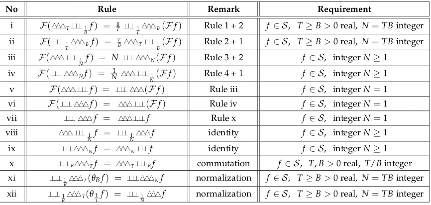
Table 2.Discrete Periodic Functions
No Rule Remark Requirement
i F(444T⊥⊥⊥1
Bf) = B T⊥⊥⊥1
T444B(Ff) Rule 1 + 2 f ∈ S, T≥B>0 real, N=TBinteger ii F(⊥⊥⊥1
T444Bf) = T
B444T⊥⊥⊥1
B(Ff) Rule 2 + 1 f ∈ S, T≥B>0 real, N=TBinteger iii F(444⊥⊥⊥1
Nf) = N⊥⊥⊥ 444N(Ff) Rule 3 + 2 f ∈ S, integerN≥1 iv F(⊥⊥⊥ 444Nf) = 1
N 444⊥⊥⊥1
N(Ff) Rule 4 + 1 f ∈ S, integerN≥1 v F(444⊥⊥⊥f) = ⊥⊥⊥ 444(Ff) Rule iii f ∈ S, integerN=1
vi F(⊥⊥⊥ 444f) = 444⊥⊥⊥(Ff) Rule iv f ∈ S, integerN=1
vii ⊥⊥⊥ 444f = 444⊥⊥⊥f Rule x f ∈ S, integerN=1
viii 444⊥⊥⊥1
Nf = ⊥⊥⊥N1444f identity f ∈ S, integerN≥1
ix ⊥⊥⊥444Nf = 444N⊥⊥⊥f identity f ∈ S, integerN≥1
x ⊥⊥⊥B444Tf = 444T⊥⊥⊥Bf commutation f∈ S, T,B>0 real, T/Binteger
xi ⊥⊥⊥1
B444T(θBf) = ⊥⊥⊥444Nf normalization f ∈ S, T≥B>0 real, N=TBinteger
xii ⊥⊥⊥1
Let us now summarize these rules in Table2. One may recall that Rules i, ii and Rules iii, iv describe the Discrete Fourier Transform (DFT) and its inverse, i.e., finite summations in contrast to the Discrete-Time Fourier Transform (DTFT) and its inverse in Rules 1, 2 and Rules 3, 4 (Table1) where we have infinite summations. The simplification of nested infinite sums actually falls into a recent research topic [67].
5. Four Fourier Transforms
The Poisson Summation Formula in its original version is commonly known to be true on Schwartz functions f ∈ S, see e.g. [12]. The next theorem extends this understanding to a validity on tempered distributions including non-integrable functions f ∈ OMand truly generalized functions f ∈ OC0.
Particular cases are the Dirac impulseδ∈ OC0in (28) and the function that is constantly 1∈ OMin (29). Theorem 1(Four Fourier Transforms reduce to one Fourier Transform). Let four Fourier transforms be defined as (32),(34),(36),(38) and let us denote the integral Fourier transform (32) as
F(f) = fˆ. (27)
It then follows that the other three Fourier transform definitions (34),(36),(38) reduce to the known rules
F(444Tf) = 1T ⊥⊥⊥1
T
ˆ
f (28)
F(⊥⊥⊥1
Tf) = T444T
ˆ
f (29)
F(⊥⊥⊥ 444Nf) = N1 444 ⊥⊥⊥1
N
ˆ
f (30)
F(444 ⊥⊥⊥1
Nf) =N⊥⊥⊥ 444N
ˆ
f (31)
where⊥⊥⊥is discretization,444is periodization, defined as in (13), (14), T>0is real, N>0an integer and (27) is the Integral Fourier TransformF (for non-discrete non-periodic functions) inS0,
(28) is the Integral Fourier TransformFper for (non-discrete) periodic functions inS0,
(29) is its inverse, the Discrete-Time Fourier Transform (DTFT) for discrete (non-per.) functions inS0, (30) is the Discrete Fourier Transform (DFT) for discrete periodic functions inS0,
(31) is its inverse, the inverse Discrete Fourier Transform (iDFT) for discrete periodic functions inS0. and the equations (27),(28),(29),(30) hold in the tempered distributions sense if
f ∈ S0=F(S0)in (27), f ∈ OC0 =F(OM)in (28), f ∈ OM=F(OC0)in (29) and f ∈ S =F(S)in (30) and (31). Furthermore,
(28) and (29) are dual generalizations of the Poisson Summation Formula (PSF) and (30) and (31) are (28) and (29) nested into one another in two different ways. Finally, for any f ∈ S, it follows that (27),(28),(29),(30),(31) hold simultaneously inS0.
Proof. The symbolic derivation of (28),(29),(30),(31) from (32),(34),(36),(38) is shown in Appendix8
and their validities inS0follow from Lemmas1-8. The circumstance that (28),(29) describe generalized variants of the Poisson summation formula is shown in Section2.4and nesting them into one another yields (30),(31) according to Lemmas7and 8. The last statement, finally, is already known [12].
Roughly, the theorem states that "instead of four Fourier transforms there is only one and instead of one Poission Summation Formula there are actually four". Let us furthermore recall that requiring
f ∈ OMin (29), which means that it is infinitely differentiable and bounded by a polynomial, is not
Mathematics2018,xx, x 11 of 19
Remark 1(Bandlimitness). In all practical cases, f is bandlimited in the sense thatFf ∈ OC0and this already fulfills the requirement f ∈ OM. Vice versa, if f ∈ O/ MthenFf ∈ O/ C0. Hence, f cannot be bandlimited. One may recall that the space of compactly supported tempered distributionsE0is a proper subspace ofOC0,
[9], p.170. The conditionFf ∈ OC0may therefore be understood as a wider comprehension of bandlimitness. 2
⊥⊥⊥ ⊥⊥⊥ DFTF
perF
DTFT DFT periodic discrete discrete periodic periodic discretenot discrete not periodic
not periodic not discrete
discrete periodic discrete periodic periodic discrete
⊥⊥⊥ ⊥⊥⊥Fig. 1. Four Fourier transforms: F, Fper, DTFT and DFT, linked via operations of discretization ⊥⊥⊥and periodization . All four transforms coincide withFin the generalized functions sense.
⊥⊥⊥ ⊥⊥ ⊥not periodic periodic
discrete not discrete periodic discrete discrete periodic
Fig. 2. Four important domains: non-discrete non-periodic functions, periodic functions, discrete functions and discrete periodic functions; linked via discretization⊥⊥⊥and periodization.
no scope whatsoever for possibly deviating definitions, i.e., all
four definitions already follow from
F
as well as ( 1) and (2).
The reason why equations (3)-(6) could not be found with
conventional means, i.e., without using an idea of
general-ized functions, is twofold. It results from the dual fact that
Lebesgue’s integral is inadequate today, in the sense that
•
it yields zero if discrete functions are integrated and
•
it yields infinity if periodic functions are integrated.
These disadvantages have been overcome in generalized
func-tions theory because it allows ”measuring” discrete and
peri-odic functions in the sense of Horv´ath’s integral [ 13].
A. Fourier Transform for periodic functions (
F
per)
In this subsection we will see that if a periodic function
is Fourier transformed via the Fourier transform for periodic
functions (9) then the result is a discrete function. Indeed,
TABLE I
DISCRETEFUNCTIONS VS. PERIODICFUNCTIONS
No Rule Remark
1 F(⊥⊥⊥1
Tf) = TT(Ff) Poisson Sum Formula 2 F(Tf) = T1 ⊥⊥⊥1
T
(Ff) Poisson Sum Formula
3 F(⊥⊥⊥f) = (Ff) abbreviated forT = 1 4 F(f) = ⊥⊥⊥(Ff) abbreviated forT = 1 5 F(⊥⊥⊥1) = (F1) whereF1 =δ
6 F(δ) = ⊥⊥⊥(Fδ) whereFδ= 1 7 F(⊥⊥⊥1) = ⊥⊥⊥1 Dirac comb invariance 8 F(δ) = δ Dirac comb invariance 9 ⊥⊥⊥T1 = Tδ Dirac comb identity 10 δ = ⊥⊥⊥1 Dirac comb identity 11 F(⊥⊥⊥1
T
1) = TTδ Dirac comb reciprocity
12 F(Tδ) = T1 ⊥⊥⊥1
T
1 Dirac comb reciprocity
13 F(f·g) = Ff∗ Fg multiplication 14 F(f∗g) = Ff· Fg convolution 15 ⊥⊥⊥g ·f=⊥⊥⊥(g·f) discretization 16 g ∗f=(g∗f) periodization 17 ⊥⊥⊥1·f=⊥⊥⊥(1·f) =⊥⊥⊥f discretization off
18 δ ∗f=(δ∗f) =f periodization off
TABLE II
DISCRETEPERIODICFUNCTIONS
No Rule Remark
i F(⊥⊥⊥1
TPf) = T
P T⊥⊥⊥1
P(Ff) Rule 1 + 2 ii F(P⊥⊥⊥1
T
f) = T P ⊥⊥⊥1
PT
(Ff) Rule 2 + 1
iii ⊥⊥⊥Nf = N⊥⊥⊥f identity
v F(⊥⊥⊥ Nf) = N1 ⊥⊥⊥1
N
(Ff) Rule 3 + 2
vi F(⊥⊥⊥1
Nf) = N⊥⊥⊥ N(Ff) Rule 4 + 1
inserting some
p(t) = (
Tf)(t)
into (9) yields
ˆ
p(m) =
1
T
T0
T
f
(t)
e
− 2πimTt
dt
=
1
T
∞−∞
f
(t)
e
−2πimTtdt
=
1
T
(
F
f
)(
m
T
)
where we used the popular periodization trick [14] and
Fourier transform definition (7). Inserting these coefficients
into (10) we obtain
(
Tf)(t) =
1
T
∞
m=−∞
(
F
f
)(
m
T
)
e
2πi tm T
=
1
T
F
−1 ∞m=−∞
(
F
f
)(
m
T
)
δ(σ
−
m
T
)
=
1
T
F
−1(
⊥⊥⊥1T
(
F
f
))(σ)
=
1
T
(
F
−1
⊥⊥⊥1
T
F
f
)(t)
(
F
(
Tf
))(σ) =
1
T
(
⊥⊥⊥T1(
F
f))(σ).
Preprints (www.preprints.org) | NOT PEER-REVIEWED | Posted: 23 May 2018 doi:10.20944/preprints201712.0173.v2
Figure 1. Four Fourier transforms and the links ⊥⊥⊥and 444between them. In the tempered
distributions sense, all four transformsF,Fper, DTFT and DFT reduce to only one Fourier transform, the Fourier transform on tempered distributions.
The interlinking formulas (28), (29), (30), (31) can be visualized in a simple diagram (Figure1). For simplicity, we use a Gaussian, i.e., a so-called self-reciprocal function [68], in order to withhold an existing reciprocity t−17→t+1 between time (left or right column) and frequency (right or left column). More generally, wide Gaussians become narrow Gaussians and narrow Gaussians become wide Gaussians. One may notice that starting from the integral Fourier transform (middle row) only Schwartz functions can reach the domain of the DFT (above and below). That is what we proved in Lemmas7and8. It is also clear that "above" and "below" coincide. Hence, the diagram is double-cyclic. Identifying the upper left side with the lower right side, we may also think of it as a Möbius band. It tells us that there is actually no left and no right-hand side, just opposite sides.
6. Discussion
The Poisson summation formula in its four variants is the actual link between the four usually defined Fourier transforms. The naming of these four Fourier transformsF,Fper, DTFT and DFT in
the literature is often not very appropriate and sometimes confusing. They should be called "Fourier transform", "Fourier transform for periodic functions", "Fourier transform for discrete functions" and "Fourier transform for discrete periodic functions" more appropriately. All four transforms moreover describe special cases of the Fourier transform on tempered distributions; they only differ in the kind of functions they are applied to, i.e., to f,444Tf,⊥⊥⊥Tf or 444N⊥⊥⊥f. An introduction of two transforms Fperand DTFT is generally not advisable because they are, apart from having an inverse sign (which
formulas should be called "Fourier Series Analysis" and "Fourier Series Synthesis" formula, as already done in many textbooks.
Furthermore it is shown that in order to be able to sample a function, it must be smooth and bounded by a polynomial. If one of these two properties is not given, the function is not bandlimited. Hence, the periodization of its Fourier transform will fail. These two conditions moreover represent a validity statement for variants of the Poisson summation formula on tempered distributions.
Remark 2(Sinc vs. Rect). The Fourier transform pair{sinc, rect}mentioned in the introduction above is a striking example for applying the validity statement for Poisson summation formula variants as discussed in this study. The equations (1) and (2) hold if g≡sinc and f ≡rect but they fail if f ≡sinc and g≡rect and the reason for this phenomenon is that
rect∈ OC0 but rect∈ O/ M and sinc∈ OM but sinc∈ O/ C0
which can easily be seen because rect is of compact support and therewith it is rapidly decreasing (∈ OC0). But it is not smooth in the ordinary functions sense (∈ O/ M). In contrast, sinc is smooth in the ordinary functions sense (∈ OM) but slowly decreasing (∈ O/ C0), it goes with1/t towards infinity which is a polynomial decrease. However, since rect∈ OC0it can be periodized and since sinc∈ OM, it can be discretized. A particular case arising from these facts is444(rect) = 1and⊥⊥⊥(sinc) = δ, respectively. Let us add them as Rule 19 and
Rule 20 in Table1.
Remark 3(Shannon’s formula fails inS0). Another consequence of this slow decrease of sinc is its failure to serve as an universal building block in Shannon’s (and Kotelnikov’s) reconstruction formula whenever we restore functions from their sampled versions. This reconstruction formula fails inS0if applied to arbitrary tempered
distributions [2]. However, instead of using the sinc function there is a wide range of other possible building blocks (Lighthill’s unitary functions [18,69]) for reconstructing tempered distributions. Unitary functions play a central role in a sampling theorem on tempered distributions. We will treat them in a future paper in greater detail.
Acknowledgments:The author would like to thank Prof. Hans G. Feichtinger for many fruitful discussions.
7. APPENDIX: Fourier Transforms
There are mainly three ways of how to deal with the factor 2πin Fourier transform definitions. Here, we use the so-called "unitary, ordinary frequency" Fourier transform as it is given for example in [2,10,12]. It is also called the "normalization" of the Fourier transform [12] because it uses 1-periodic exponential functionse2πiσrather than 2π-periodic oneseiσand thereby yields the most symmetric
results in Fourier transform pairs, e.g.Fδ=1 andF1=δ. The normalized Fourier transform actually linksZtoRvia 1-periodic functions. As a result of this, "time domain" and "frequency domain" become
fully equivalent.
7.1. Conventional Fourier Transforms
Mathematics2018,xx, x 13 of 19
7.1.1. Fourier Transform
The Integral Fourier Transform (for non-discrete non-periodic functions) is defined by
ˆ
f(σ) =
Z ∞
−∞f(t)e
−2πitσdt Analysis (32)
f(t) = Z ∞
−∞
ˆ
f(σ)e2πiσtdσ Synthesis (33)
for suitablef(t).
7.1.2. Fourier Transform (for periodic functions)
The Integral Fourier Transform for (non-discrete) periodic functions, used forFourier Series
analysis, is defined by
ˆ
f[m] = 1 T
Z T
0 f(t)e
−2πiTtmdt Analysis (34)
f(t) =
∑
∞ m=−∞ˆ
f[m]e2πimTt Synthesis (35)
where (35) is theFourier Seriesof f(t)and (34) determines its coefficients. The coefficients arediscrete. 7.1.3. Fourier Transform (for discrete functions)
The Fourier Transform for discrete (non-periodic) functions, also calledDiscrete-Time Fourier Transform(DTFT), used forFourier Seriessynthesis, is defined by
ˆ
f(σ) = 1
T ∞
∑
k=−∞f[k]e−2πiTkσ Analysis (36)
f[k] = Z T
0
ˆ
f(σ)e2πi
σ
Tkdσ Synthesis (37)
where (36) is aFourier Series. Hence, it isperiodicbut f(t)itself isdiscrete, its samples are determined by (37).
7.1.4. Fourier Transform (for discrete periodic functions)
The Fourier Transform for discrete periodic functions, calledDiscrete Fourier Transform(DFT) is defined by
ˆ
f[m] = 1 N
N−1
∑
k=0f[k]e−2πiNkm Analysis (38)
f[k] = N−1
∑
m=0ˆ
f[m]e2πimNk Synthesis (39)
where both, (38) and (39), are (finite-sum) Fourier Series. Thus, they are periodic and discrete, simultaneously.
7.2. Distributional Fourier Transform
Lethf,ϕibe the application of a tempered distribution f ∈ S0to some test functionϕ∈ S. The Fourier transform of f ∈ S0is then defined as
whereF on the right-hand side is the integral Fourier transform given by (32) and its inverse is (33), respectively. One usually uses this definition to test and verify symbolic calculation rules on tempered distributions. Once the rules are established, they can symbolically be used on tempered distributions as if they were ordinary functions. It is known that Fourier transform rules which apply to Lebesgue-square integrable functions do also apply to tempered distributions. Additionally, new rules can be found such asF1= δandFδ=1 which are based on rigorous calculations using the above definition. Rules summarized in Table1were established in [6]. They do also hold on ordinary square-integrable functions under the same conditions.
Most convenient is the fact that using the Fourier transform in the distributional sense, all functions become infinitely differentiable. In other words, the Fourier transform rule "multiplying a function k times with 2πitin one domain means to differentiate its Fourier transform k times in the other domain", e.g. in [2,5,10,26,28,60], can be exploited unrestrictedly. One may recall that 2πitis the inner derivative ofe2πitσ. It means, the Fourier transform rule originates from
d dσ e
2πitσ = (2πit)e2πitσ
becausee2πitσis infinitely differentiable in the ordinary functions sense. The special role ofe2πitσarises
from the fact that it is a number and a function, simultaneously.
8. APPENDIX: Derivations
In this appendix, we symbolically derive (28),(29),(30),(31) from four definitions of the Fourier transform given in (32),(34),(36),(38). We prove that
• defining the Integral Fourier Transform for periodic functions via (34),(35) leads to (28), • defining the Discrete-Time Fourier Transform (DTFT) via (36),(37) leads to (29) and • defining the Discrete Fourier Transform (DFT) via (38),(39) leads to (30) and (31).
Interesting is the fact that there has obviously been no other choice than defining all four Fourier transforms in exactly this way.
8.1. Fourier Transform for periodic functions (Fper)
In this subsection we will see that if aperiodic functionis Fourier transformed via the Fourier transform for periodic functions (34) then the result is adiscrete function. Indeed, inserting some
p(t) = (444Tf)(t)into (34) yields
ˆ
p(m) = 1 T
Z T
0 444Tf(t)e
−2πimTtdt
= 1 T
Z ∞
−∞ f(t)e
−2πimTtdt
= 1 T (Ff)(
Mathematics2018,xx, x 15 of 19
where we used the popularperiodization trick [13] and Fourier transform definition (32). Inserting these coefficients into (35) we obtain
(444Tf)(t) = 1 T
∞
∑
m=−∞(Ff)( m T)e
2πi tmT
= 1 T F
−1
( ∞
∑
m=−∞(Ff)( m T)δ(σ−
m T)
)
= 1 T F
−1n(⊥⊥⊥ 1
T(Ff))(σ) o
= 1 T (F
−1 ⊥⊥⊥1
TFf)(t) (F(444Tf))(σ) = 1
T (⊥⊥⊥1T(Ff))(σ).
Therefore, (34) inserted into (35) reduces to
F(444Tf) = 1
T ⊥⊥⊥1T(Ff)
as a function ofσ∈R. This is formula (28).
8.2. Fourier Transform for discrete functions (DTFT)
We show that if adiscrete functionis Fourier transformed via the DTFT then the result is aperiodic function. As (36) is a Fourier series, it is periodic. The ansatz is therefore to let ˆd(σ) = (444Tfˆ)(σ) =
(444T(Ff))(σ)in (37). It yields
d(k) = Z T
0 444T
ˆ
f(σ)e2πi
k Tσdσ =
Z ∞
−∞ fˆ(σ)e 2πikTσd
σ
= (F−1(Ff))(k
T) = f( k T).
Inserting these coefficients into (36) we obtain
(444T(Ff))(σ) = 1
T ∞
∑
k=−∞f(k T)e−
2πiσkT
= 1 T F
( ∞
∑
k=−∞f(k T)δ(t−
k T)
)
= 1 T F
n (⊥⊥⊥1
Tf)(t) o
= 1
T (F(⊥⊥⊥1Tf))(σ).
Thus, (37) inserted into (36) reduces to F(⊥⊥⊥1
Tf) =T444T(Ff)
as a function ofσ∈R. This is formula (29).
8.3. Fourier Transform for discrete periodic functions (DFT)
function(444Tf)(t)it can be denoted asy(t) = (⊥⊥⊥444Nf)(t)whereNis an integer corresponding to its periodT. Inserting now its coefficients(444Nf)(k)withk∈Zinto (38) yields
(F(444Nf))(m) = 1 N
N−1
∑
k=0(444Nf)(k)e−2πimNk
= 1 N
∞
∑
k=−∞f(k)e−2πimNk
= 1
N (F(⊥⊥⊥f))( m N) = 1
N (444(Ff))( m N)
using, again, the periodization trick (applied to a discrete function this time), the definition of discretization⊥⊥⊥and a previous result (Rule 4). Inserting these coefficients into (39) we obtain
(444Nf)(k) = 1 N
N−1
∑
m=0444 (Ff)(m N)e
2πi kmN
= 1 N
∞
∑
m=−∞ (F f)(m
N)e 2πi kmN
= 1 N (F
−1 ⊥⊥⊥1
N(Ff))(k).
again with the periodization trick, discretization⊥⊥⊥and the definition ofF−1this time. Thus, (38)
inserted into (39) reduces to
(444Nf)(k) = 1
N (F
−1 ⊥⊥⊥1
N(Ff))(k), k∈Z (⊥⊥⊥ 444Nf)(t) = 1
N (⊥⊥⊥F
−1 ⊥⊥⊥1
N(Ff))(t), t∈R
and with Rule 4 and Fourier transforming both sides it yields
F(⊥⊥⊥ 444Nf) = 1
N 444 ⊥⊥⊥N1(Ff)
being a function ofσ∈R.
8.4. Derivation of the Inverse DFT
As (38) is a Fourier series, it is periodic. Evaluating (39) for ˆg(m) = (444Nfˆ)(m)where ˆf =Ff
yields
g(k) = N−1
∑
m=0(444N(Ff))(m)e2πiNkm
=
∑
∞ k=−∞(Ff)(m)e2πiNkm
= (F−1
⊥⊥⊥(Ff))(k N) = (F−1F(444f))(k
N) = (444f)( k
Mathematics2018,xx, x 17 of 19
and inserting this result into (38) we obtain
(444N(Ff))(m) = 1 N
N−1
∑
k=0(444f)( k N)e−
2πi mNk
= 1 N
∞
∑
k=−∞f(k N)e−
2πi mNk
= 1
N (F(⊥⊥⊥N1 f))(m).
Thus, (39) inserted into (38) reduces to
(F(⊥⊥⊥1
Nf))(m) =N(444N(Ff))(m), m∈Z (⊥⊥⊥F(⊥⊥⊥1
Nf))(σ) =N(⊥⊥⊥ 444N(Ff))(σ), σ∈R
and with Rule 4 on the left hand side it yields
F(444 ⊥⊥⊥1
Nf) =N⊥⊥⊥ 444N(Ff)
being a function ofσ∈R.
Altogether, we proved that the Discrete Fourier Transform (DFT) together with its inverse follow these two rules
F(⊥⊥⊥ 444Nf) = 1
N 444 ⊥⊥⊥N1(Ff) and
1
N F(444 ⊥⊥⊥N1f) = ⊥⊥⊥ 444N(Ff)
as functions ofσ∈R, which are (30) and (31), respectively.
Conflicts of Interest:The author declares no conflicts of interest.
References
1. Woodward, P.M.Probability and Information Theory, with Applications to Radar; Pergamon Press, 1953. 2. Gasquet, C.; Witomski, P. Fourier Analysis and Applications: Filtering, Numerical Computation, Wavelets;
Vol. 30, Springer Science & Business Media, 1999.
3. Panaretos, A.H.; Anastassiu, H.T.; Kaklamani, D.I. A Note on the Poisson Summation Formula and Its Application to Electromagnetic Problems Involving Cylindrical Coordinates.Turkish Journal of Electrical Engineering & Computer Sciences2002,10, 377–384.
4. Benedetto, J.J.; Zimmermann, G. Sampling Multipliers and the Poisson Summation Formula. Journal of Fourier Analysis and Applications1997,3, 505–523.
5. Strichartz, R.S.A Guide to Distribution Theorie and Fourier Transforms; World Scientific, 2003.
6. Fischer, J. Anwendung der Theorie der Distributionen auf ein Problem in der Signalverarbeitung. Diploma thesis, Ludwig-Maximillians-Universität München, Fakultät für Mathematik, 1997.
7. Halperin, I.; Schwartz, L.Introduction to the Theory of Distributions; University of Toronto Press, 1952. 8. Schwartz, L.Théorie des Distributions, Tome I; Hermann Paris, France, 1950.
9. Schwartz, L.Théorie des Distributions, Tome II; Hermann Paris, France, 1951.
10. Kammler, D.W.A First Course in Fourier Analysis; Cambridge University Press, 2007. 11. Benedetto, J.J.Harmonic Analysis and Applications; Vol. 23, CRC Press, 1996.
12. Feichtinger, H.G.; Strohmer, T.Gabor Analysis and Algorithms: Theory and Applications; Springer, 1998. 13. Gröchenig, K.Foundations of Time-Frequency Analysis; Birkhäuser, 2001.
14. Brandwood, D.Fourier Transforms in Radar and Signal Processing; Artech House, 2003. 15. Rahman, M.Applications of Fourier Transforms to Generalized Functions; WIT Press, 2011.
17. Temple, G. The Theory of Generalized Functions. Proceedings of the Royal Society of London. Series A. Mathematical and Physical Sciences1955,228, 175–190.
18. Lighthill, M.J.An Introduction to Fourier Analysis and Generalised Functions; Cambridge University Press, 1958.
19. Zemanian, A.Distribution Theory And Transform Analysis - An Introduction To Generalized Functions, With Applications; McGraw-Hill, 1965.
20. Trèves, F.Topological Vector Spaces, Distributions and Kernels: Pure and Applied Mathematics; Vol. 25, Dover Publications Inc, Mineola, New York, 1967.
21. Horváth, J.Topological Vector Spaces and Distributions; Addison-Wesley Publishing Company, 1966. 22. Jones, D.The Theory of Generalized Functions; Cambridge University Press, 1966.
23. Zemanian, A.H.Generalized Integral Transformations; John Wiley & Sons, Inc., 1968. 24. Barros-Neto, J.An Introduction to the Theory of Distributions; Dekker, 1973.
25. Wagner, P. Zur Faltung von Distributionen.Mathematische Annalen1987,276, 467–485.
26. Hörmander, L. The Analysis of Linear Partial Differential Operators I, Die Grundlehren der mathematischen Wissenschaften; Springer, 1983.
27. Walter, W.Einführung in die Theorie der Distributionen; BI-Wissenschaftsverlag, Bibliographisches Institut & FA Brockhaus, 1994.
28. Vladimirov, V.Methods of the Theory of Generalized Functions, CRC Press, 2002.
29. Fischer, J.V. On the Duality of Discrete and Periodic Functions. Mathematics2015,3, 299–318. 30. Fischer, J.V. On the Duality of Regular and Local Functions.Mathematics2017,5, 41.
31. Constantinescu, F.Distributions and Their Applications in Physics: International Series in Natural Philosophy; Vol. 100, Elsevier, 1980.
32. Saichev, A.I.; Woyczynski, W.A.Distributions in the Physical and Engineering Sciences. Volume 2 - Linear and Nonlinear Dynamics of Continuous Media; Birkhäuser-Boston, 2013.
33. Messiah, A. Quantum Mechanics – Two Volumes Bound as One, 2003.
34. Glimm, J.; Jaffe, A.Quantum Physics: A Functional Integral Point of View; Springer Science & Business Media, 2012.
35. Debnath, L. A Short Biography of Paul A M Dirac and Historical Development of Dirac Delta Function.
International Journal of Mathematical Education in Science and Technology2013,44, 1201–1223. 36. Dirac, P.The Principles of Quantum Mechanics; Oxford University Press, 1930.
37. Dierolf, P. The Structure Theorem for Linear Transfer Systems. Note di Matematica1991,11, 119–125. 38. Smith, D.C. An Introduction to Distribution Theory for Signals Analysis. Digital Signal Processing2006. 39. Unser, M. Sampling-50 Years after Shannon. Proceedings of the IEEE2000,88, 569–587.
40. Grossmann, A.; Loupias, G.; Stein, E.M. An Algebra of Pseudodifferential Operators and Quantum Mechanics in Phase Space. Ann. Inst. Fourier1968,18, 343–368.
41. Taylor, M.E. Pseudodifferential operators. InPartial Differential Equations II; Springer, 1996; pp. 1–73. 42. Ashino, R.; Boggiatto, P.; Wong, M.W.Advances in Pseudo-Differential Operators; Vol. 155, Birkhäuser, 2012. 43. Feichtinger, H.G.Modulation Spaces on Locally Compact Abelian Groups; Universität Wien. Mathematisches
Institut, 1983.
44. Gröchenig, K.; Heil, C. Modulation Spaces and Pseudodifferential Operators. Integral Equations and Operator Theory1999,34, 439–457.
45. Bényi, Á.; Gröchenig, K.; Okoudjou, K.A.; Rogers, L.G. Unimodular Fourier Multipliers for Modulation Spaces. Journal of Functional Analysis2007,246, 366–384.
46. Feichtinger, H.G. On a New Segal Algebra. Monatshefte für Mathematik1981,92, 269–289.
47. Özça ˘g, E. Defining the k-th Powers of the Dirac-Delta Distribution for Negative Integers. Applied Mathematics Letters2001,14, 419–423.
48. Li, C. The Powers of the Dirac Delta Function by Caputo Fractional Derivatives. Journal of Fractional Calculus and Applications2016,7, 12–23.
49. Bracewell, R.N.Fourier Transform and its Applications; McGraw-Hill Education, 1986.
Mathematics2018,xx, x 19 of 19
51. Gracia-Bondía, J.M.; Varilly, J.C. Algebras of Distributions Suitable for Phase-Space Quantum Mechanics. I.
Journal of Mathematical Physics1988,29, 869–879.
52. Dubois-Violette, M.; Kriegl, A.; Maeda, Y.; Michor, P.W. Smooth*-Algebras. arXiv preprint math/0106150
2001.
53. Ortner, N. On Convolvability Conditions for Distributions.Monatshefte für Mathematik2010,160, 313–335. 54. Larcher, J. Multiplications and Convolutions in L. Schwartz’ Spaces of Test Functions and Distributions
and their Continuity. Analysis2013,33, 319–332. 55. Ortner, N.; Wagner, P. On the SpacesOm
C of John Horváth. Journal of Mathematical Analysis and Applications
2014,415, 62–74.
56. Katznelson, Y. Une remarque concernant la formule de Poisson. Studia Mathematica1967,29, 107–108. 57. Butzer, P.L.; Stens, R. The Poisson Summation Formula, Whittaker’s Cardinal Series and Approximate
Integration. Second Edmonton conference on approximation theory. Amer. Math. Soc. Providence, RI, 1983, pp. 19–36.
58. Kahane, J.P.; Lemarié-Rieusset, P.G. Remarques sur la formule sommatoire de Poisson. Studia Math1994,
109, 303–316.
59. Gröchenig, K. An Uncertainty Principle related to the Poisson Summation Formula.Studia Mathematica
1996,121, 87–104.
60. Nguyen, H.Q.; Unser, M.; Ward, J.P. Generalized Poisson Summation Formulas for Continuous Functions of Polynomial Growth. Journal of Fourier Analysis and Applications2017,23, 442–461.
61. Lyness, J. The Calculation of Fourier Coefficients by the Möbius Inversion of the Poisson Summation Formula. I. Functions whose early derivatives are continuous. Mathematics of Computation1970,24, 101–135. 62. Kerl, J. Poisson Summation and the Discrete Fourier Transform2008.
63. Feichtinger, H.G. Thoughts on Numerical and Conceptual Harmonic Analysis. InNew Trends in Applied Harmonic Analysis; Springer, 2016; pp. 301–329.
64. Susskind, L.; Friedman, A.Quantum Mechanics: The Theoretical Minimum; Basic Books, 2014.
65. Baggott, J.The Meaning of Quantum Theory: A Guide for Students of Chemistry and Physics; Oxford University Press, New York, 1992.
66. Arici, F.; Becker, D.; Ripken, C.; Saueressig, F.; van Suijlekom, W.D. Reflection Positivity in Higher Derivative Scalar Theories.Journal of Mathematical Physics2018,59, 082302.
67. Paule, P.; Schneider, C. Towards a Symbolic Summation Theory for Unspecified Sequences.arXiv preprint arXiv:1809.065782018.
68. Born, M. Reciprocity Theory of Elementary Particles. Reviews of Modern Physics1949,21, 463.
69. Boyd, J.P. Construction of Lighthill’s Unitary Functions: The Imbricate Series of Unity. Applied Mathematics and Computation1997,86, 1–10.
c