An efficient local formulation for time–dependent
PDEs
Imtiaz Ahmad
a, Muhammad Ahsan
a,b, Masood Ahmad
b,
Zaheer-ud-Dinb and Poom Kumamc,∗aDepartment of Mathematics, University of Swabi, Swabi, Pakistan
bDepartment of Basic Sciences, University of Engineering and Technology, Peshawar, Pakistan
dKMUTTFixed Point Research Laboratory, Room SCL 802 Fixed Point Laboratory, Department of Mathematics, Science
Laboratory Building, Faculty of Science, King Mongkut’s University of Technology Thonburi (KMUTT), 126 Pracha-Uthit
Road, Bang Mod, Thrung Khru, Bangkok 10140, Thailand
Abstract
In this paper, a local meshless method (LMM) based on radial basis functions (RBFs) is utilized for the numerical solution of various types of PDEs, due to the flexibility with respect to geometry and high order of convergence rate. In case of global meshless methods, the two major deficiencies are the computational cost and the optimum value of shape parameter. Therefore, research is currently focus towards localized radial basis function approximations, as the local meshless method is proposed here. The local meshless procedures is used for spatial discretization whereas for temporal discretization different time integrators are employed. The proposed local meshless method is testified in terms of efficiency, accuracy and ease of implementation using regular and irregular domains.
Keywords: Local meshless method, RBFs, Irregular domains, Kortewege-de Vries types
equations, reaction-diffusion Brusselator system.
1
Introduction
Most of the problems in real world can be described by partial differential equations (PDEs). In this regard one of the important PDE model is fifth order Kortewege-de Vries model. Its general exact solution is not known whereas the exact solution for particular case of solitary waves can
be found in [48]. To solve this model numerically, serval methods can be found in literature
such as finite–deference scheme [13], modified ADM [8], decomposition method [27], Homotopy
perturbation transform method [18] and a comparative study of Crank-Nicolson method and
ADM [21].
The general seventh order Kortewege-de Vries equation [34] which is used to discuss structural
stability under singular perturbation of standard KdV equation. Several authors have paid
attention to solve the seventh order KdV equation [12,14,40].
Generalized Burgers’ Huxley equation [35] is used to describe the interaction between convection
effects, reaction mechanisms and diffusion transports. In general it is difficult and sometimes impossible to get exact solution of such type nonlinear PDE. Researchers employed different
numerical techniques which include discrete Adomian decomposition method [4], Haar wavelet
method [11], Adomian decomposition method [24], meshless collocation method based on RBF
[29] and local meshless method [10] for the solution of Burgers’ Huxley equation. The Huxley
model equation [23] describes nerve pulse propagation in nerve fibres and wall motion in liquid
crystals [7]. Numerical solution of Huxley equation can be found in [5,24,29] and the references
therein. Generalized Burgers’ Fisher equation [15], describe the propagation of a mutant gene.
Different numerical methods have been used for numerical solution of this model, such as meshless
collocation method [29], ADM [24], VIM [32], modified pseudo spectral method [25] and modified
cubic B–spline functions collocation method [31].
The Fitzhugh-Nagumo (FN) equation has numerous applications in different fields such as branching brownian motion process, flame propagation, neurophysiology, logistic population
growth and nuclear reactor theory [9]. Numerical solution of FN equation can be found in
[1,20,26,31].
Hirota-Satsuma introduced the nonlinear coupled Kortewege–de Vries equations [22]. This model
has numerous applications in physical sciences. In the last decade, researchers have used various numerical techniques for the solution of this model equations. These include RBFs collocation
(Kansa) method [39], meshless RBFs method of lines [19], variational iteration method [6] and
spectral collocation method [28]. The Hirota–Satsuma coupled KdV system [47] has been solved
by different numerical methods given in [17,28,43] and the references therein.
The Brusselator system is one of the essential reaction–diffusion model equation. This model
explain the mechanism of a chemical reaction–diffusion with non–linear oscillations [30,42].
Nu-merical solution of the model can be found in [2,38,45,46].
In the last few years, it is observed that meshless methods have been extensively employed
for numerical simulations of different types of PDEs [37,39,41]. Meshless methods reduce
com-plexity caused due to dimensionality to a large extent which is being faced in the carrying out of conventional methods like finite-element and finite-difference procedures. Meshing in the case of complicated geometries is another cause for the growing demand of meshless methods.
It is noticed that global meshless methods faced the problem of dense ill-conditioned matrices and finding optimum value of the shape parameter. To avoid these problems, local meshless
methods are used as alternative to get a stable and accurate solution for the PDE models [3,37].
2
Partial differential equation models
A short description of PDE models on a bounded domain with corresponding initial and boundary conditions are given in this section. These include; one-dimensional fifth order Lax’s-Kortewege-de Vries, seventh orLax’s-Kortewege-der Lax’s-Kortewege-Lax’s-Kortewege-de Vries, generalized Burgers’-Huxley, Huxley, gener-alized Burgers’ Fisher, Fitzhugh-Nagumo, coupled Kortewege-de Vries, Hirota-Satsuma coupled Kortewege-de Vries equations and two-dimensional reaction-diffusion Brusselator equations.
The 1D fifth order Kortewege-de Vries equation [8],
Ut+aU2Ux+bUxUxx+cU Uxxx+dUxxxxx= 0, (1)
wherea,b,c,dare real constants and in this paper we have taken a=b= 30,c= 10, andd= 1.
The 1D seventh order Kortewege-de Vries equation [12],
Ut+aU3Ux+bUx3+cU UxUxx+dU2Uxxx+eUxxUxxx+f UxUxxxx+gU Uxxxxx+Uxxxxxxx= 0, (2)
wherea, b,c, d, e, f, g are real constants and we have taken a= 140, b = 70,c = 280, d= 70,
The 1D generalized Burgers’-Huxley equation [4,11,24,29,35],
Ut+αUδUx−Uxx−βU(1−Uδ)(Uδ−γ) = 0, (3)
whereα,β≥0, δ >0, γ∈(0,1) are constants.
The 1D Huxley equation [5,24,29]
Ut−Uxx−βU(1−U)(U−γ) = 0, (4)
whereβ andγ are constants.
The 1D generalized Burgers’ Fisher equation [24,29],
Ut+αUδUx−Uxx−βU(1−Uδ) = 0, (5)
whereα,β and δ are constants.
The 1D Fitzhugh-Nagumo (FN) equation [9,16,26,33],
Ut−Uxx+U(1−U)(ρ−U) = 0, (6)
whereρ is a constant.
The 1D coupled Kortewege-de Vries equation [19,22,28,39],
Ut+ 6αU Ux−2γV Vx+αUxxx= 0,
Vt+ 3βU Vx+βVxxx= 0,
(7)
whereα,β and γ are real parameters.
The 1D Hirota-Satsuma coupled KdV system of equations [28,47],
Ut−
1
2Uxxx+ 3U Ux−3V Wx−3W Vx = 0,
Vt+Vxxx−3U Vx = 0,
Wt+Wxxx−3U Wx = 0.
(8)
The 2D reaction-diffusion Brusselator system of equations [38,46]
Ut−β−U2V + (α+ 1)U −γ(Uxx+Uyy) = 0,
Vt−αU+U2V −γ(Vxx+Vyy) = 0,
(9)
whereα,β and γ are constants.
3
Local meshless numerical scheme
To pursue the LMM [36,37], we approximate the derivatives ofU(x, t) at the centerxpby the
func-tion values at a set of nodes in the neighborhood ofxp,{xp1, xp2, xp3, ..., xpnj} ⊂ {x1, x2, . . . , xNn}, np
Nn, wheren= 1,n= 2 for one and two dimensional case respectively.
U(m)(xp)≈ np
X
k=1
λ(km)U(xpk), p= 1,2, . . . , N
To find the corresponding coefficientλ(km), radial basis function φ(kx−xlk) can be substituted
into equation (10)
φ(m)(kxp−xlk) = np
X
k=1
λ(pmk)φ(kxpk−xlk), l=p1, p2, . . . , pnp. (11)
Equation (11) in matrix form
φ(pm1)(xp)
φ(pm2)(xp) .. .
φ(pmnp)(xp)
=
φp1(xp1) φp2(xp1) · · · φpnp(xp1)
φp1(xp2) φp2(xp2) · · · φpnp(xp2) ..
. ... . .. ...
φp1(xpnp) φp2(xpnp) · · · φpnp(xpnp)
λ(pm1)
λ(pm2) .. .
λ(pmnp)
, (12) where
φl(xk) =φ(kxk−xlk), l=p1, p2, . . . , pnp, (13)
for each k=p1, p2, . . . , pnp.
The above equation in matrix notation
Φ(nmp)=Anpλ (m)
np , (14)
where
Φn(mp)=h φp(m1)(xp) φ (m)
p2 (xp) · · · φ (m)
pnp(xp)
iT
Anp =
φp1(xp1) φp2(xp1) · · · φpnp(xp1)
φp1(xp2) φp2(xp2) · · · φpnp(xp2) ..
. ... . .. ...
φp1(xpnp) φp2(xpnp) · · · φpnp(xpnp)
λ(nmp) =h λ(pm1) λ (m)
p2 · · · λ (m)
pnp
iT
.
From equation (14),
λ(nmp)=An−1pΦ(nmp). (15)
By substituting equation (15) into equation (10),
U(m)(xp) = (λ(nmp))
TU
np, (16)
where
Unp =
h
U(xp1), U(xp2), . . . , U(xpnp)
iT
. (17)
3.1 1D fifth order Kortewege-de Vries equation
The 1D fifth order Kortewege-de Vries equation (1) can be written as
Ut=−(aU2Ux+bUxUxx+cU Uxxx+dUxxxxx), x∈Ω, t≥0, (18)
subject to initial and boundary conditions
U(x, t) =f1(t), U(x, t) =f2(t), x∈∂Ω. (20)
wherea,b,cand dare constants.
Now, Applying the LMM to equation (18) we get,
dUp
dt =−(aU
2
p(λ(1)np)
TU
np+b((λ (1)
np)
TU np)((λ
(2)
np)
TU
np) +cUp(λ (3)
np)
TU
np+d(λ (5)
np)
TU
np), p= 2,3, . . . , N−1.
(21)
The semi-discretized model equation (21) with boundary conditions (20) is given as follows
dU
dt =−(aU
2∗(Λ(1)U) +b(Λ(1)U)∗(Λ(2)U) +cU∗(Λ(3)U) +d(Λ(5)U)), (22)
where the symbol∗ represent element-wise multiplication of two vectors.
U= [U1, U2, U3, . . . , UN]T,
Λ(1)N×N = [mpk] = [λ
(1)
k ], k=p1, p2, . . . , pnp, p= 2,3, . . . , N−1,
Λ(2)N×N = [mpk] = [λ
(2)
k ], k=p1, p2, . . . , pnp, p= 2,3, . . . , N−1.
Λ(3)N×N = [mpk] = [λ(3)k ], k=p1, p2, . . . , pnp, p= 2,3, . . . , N−1.
Λ(5)N×N = [mpk] = [λ(5)k ], k=p1, p2, . . . , pnp, p= 2,3, . . . , N−1.
(23)
The corresponding initial condition is given as
U(t0) = [U0(x1), U0(x2), . . . , U0(xN)]T. (24)
4
Results and discussion
To check the accuracy and efficiency of the LMM various test problems in one and two dimen-sional cases are considered and the results are compared with the existence methods reported in literature. For spatial discretization three types of RBFs that is, MQ, IMQ and GA are used whereas for time integration have used explicit Euler method (EEM) and Runge-Kutta method of order 4 (RK4).
Accuracy of the LMM is measured though different error norms given as follows
Labs=|Uexact(p)−U(p)|, p= 1,2, . . . , Nn. L∞= max (Labs),
L2=
h N X
p=1
Labs2
1 2
, Lrms=
1
N
N X
p=1
Labs2
1 2
,
(25)
where exact and numerical solution are represented byUexact and U respectively.
Summary of numerical results is given as: Results of 1D fifth order KdV equation are shown
in Table 1 and compared with the method in [8] whereas numerical results of seventh order
KdV equation are presented in Table 2. Similarly the numerical results of generalized Burgers’
Huxley equation are presented in Tables 3-4 and the results are compared with the methods
given in [4,11,24,29] while the numerical results of Huxley equation are shown in Tables 5-6
and compared with the methods in [5,24,29]. Numerical results of generalized Burgers’ Fisher
Table 1: Numerical results the LMM for Test Problem1.
t EEM [8] EEM [8] EEM [8] EEM [8]
x=0.2 x=0.6 x=1 x=5
2 5.2899e-15 5.7619e-14 1.5870e-14 1.7278e-13 2.6450e-14 2.8786e-13 1.2669e-13 1.4210e-12 4 1.0580e-14 1.1528e-13 3.1740e-14 3.4561e-13 5.2900e-14 5.7577e-13 2.5337e-13 2.8421e-12 6 1.5869e-14 1.7298e-13 4.7610e-14 5.1848e-13 7.9350e-14 8.6372e-13 3.8006e-13 4.2632e-12 8 2.1159e-14 2.3073e-13 6.3479e-14 6.9140e-13 1.0580e-13 1.1517e-12 5.0676e-13 5.6844e-12 10 2.6448e-14 2.8851e-13 7.9349e-14 8.6435e-13 1.3225e-13 1.4397e-12 6.3345e-13 7.1056e-12
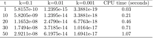
Table 2: Numerical results in form ofL∞ error norm using the EEM for Test Problem 2.
t k=0.1 k=0.01 k=0.001 CPU time (seconds)
1 5.8157e-10 1.2395e-15 3.3881e-19 0.03 10 5.8205e-09 1.2395e-14 3.3881e-18 0.21 20 1.1652e-08 2.4790e-14 6.7763e-18 0.46 30 1.7494e-08 3.7185e-14 1.0164e-17 0.71 50 2.9211e-08 6.1975e-14 1.6941e-17 1.07
Fitzhugh-Nagumo equation are given in Table8, Figs. 1-2and the results are compared with the
method reported in [26]. Numerical results of coupled KdV equations are presented in Tables 9
and the results are compared with the method given in [39] while numerical results of
Hirota-Satsuma coupled KdV equation are shown in Table10. Numerical simulation of reaction-diffusion
Brusselator system are shown in Table11 and comparison is made with the methods in [38,46].
Test Problem 1. The exact solution [8] of the 1D Lax’s fifth order KdV equation (1) is
U(x, t) = 2k2 2−3 tanh2 k(x−56k4t−x0)
, x∈[−10,10], t≥0 (26)
where the initial and boundary conditions are extracted from the exact solution (26).
Numerical results for Test Problem 1 are given in Table 1 using k = 0.01, x0 = 0, dt = 0.01,
N = 11 and shape parameterc= 100. Table 1indicated that the results produced by the LMM
using EEM are more better than the method in [8].
Test Problem 2. The 1D Lax’s seventh order KdV equation (2) having exact solution [12]
U(x, t) = 2k2sech2 k(x−64k6t)
, x∈[−100,100], t≥0 (27)
where the initial and boundary equations are extracted from the exact solution (27).
To demonstrate the accuracy and efficiency of the proposed LMM, we reported numerical results
in Table 2 for Test Problem 2, in form of L∞ error norm using different values of k and t. We
have used EEM withdt= 0.01,N = 11 using MQ RBF (c= 100). From Table2, one can observe
that the LMM is accurate and efficient.
Test Problem 3. The 1D generalized Burgers’ Huxley equation (3) having exact solution taken
from [44] is given by
U(x, t) =
γ
2 +
γ
2tanh (ω1(x−ω2t))
1δ
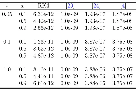
Table 3: Numerical results of generalized Burgers’ Huxley equation in term of Labs error norm using the RK4 for Test Problem3.
t x RK4 [29] [24] [4]
0.05 0.1 6.30e-12 1.0e-09 1.93e-07 1.87e-08 0.5 4.42e-12 1.0e-09 1.93e-07 1.87e-08 0.9 2.55e-12 1.0e-09 1.93e-07 1.87e-08
0.1 0.1 1.23e-11 1.0e-09 3.87e-07 3.75e-08 0.5 8.62e-12 1.0e-09 3.87e-07 3.75e-08 0.9 4.87e-12 1.0e-09 3.87e-07 3.75e-08
1.0 0.1 8.16e-11 0.0e-09 3.88e-06 3.75e-07 0.5 4.41e-11 0.0e-09 3.88e-06 3.75e-07 0.9 6.61e-12 0.0e-09 3.88e-06 3.75e-07
where
ω1=
−αδ+δpα2+ 4β(1 +δ)
4(1 +δ) γ, ω2 =
αγ
1 +δ −
(1 +δ−γ)(−α+pα2+ 4β(1 +δ))
2(1 +δ) ,
whereα,β,δ and γ are constants such thatβ≥0,δ >0,γ ∈(0,1).
In Table3, we have compared the results obtained by the LMM for generalized Burgers’ Huxley
equation for Test Problem 3with the methods given in [4,24,29]. We have used the parameters
values α=β =δ = 1 andγ = 0.001 and time step lengthdt = 0.0001, spatial domain [−10,20],
N = 61 using IMQ RBF. From Table 3, we have noted that the RK4 produced more accurate
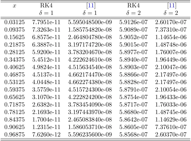
results than the results reported in [4,24,29]. Table 4 also shows the comparison of numerical
results produced by the LMM with the results of Haar wavelet method given in [11]. In the table
we have calculated the absolute errors for different values ofxand δ with α=β = 1,γ = 0.001,
and t= 0.8 using IMQ RBF. It can be observed from the table that the LMM is more accurate
than the method reported in [11]. The numerical results of Huxley equation for Test Problem
3 with spatial domain [−10,20], N = 61, dt = 0.01 and different values of x and t are shown
in Table 5. We have used IMQ radial basis function and β =δ = 1, γ = 0.001. The numerical
simulations have carried out by using the RK4 and comparison is done with [24,29] in Table
5. From the table, we have noticed that the results produced by the LMM are better than the
methods reported in [24,29].
Test Problem 4. The exact solution [7] of the 1D Huxley equation (4) with α=γ = 1 is given
below as
U(x, t) =1
2 +
1
2tanh
1 2√2(x−
t
√ 2)
, a≤x≤b, t≥0, (29)
The numerical simulations have carried out for Test Problem 4in Table 6for different values of
t, x, a, b and for N = 10, dt = 0.0001 using MQ RBF with c = 5. The results are obtained
by the EEM and compared with the results obtained by Chebyshev spectral collocation method
Table 4: Numerical results in form ofLabs error norm using the RK4 for Test Problem3.
x RK4 [11] RK4 [11]
δ= 1 δ= 1 δ= 2 δ= 2
0.03125 7.7951e-11 5.595048500e-09 5.9126e-07 2.60170e-07 0.09375 7.3263e-11 1.585754820e-08 5.9089e-07 7.37310e-07 0.15625 6.8575e-11 2.464804780e-08 5.9052e-07 1.14654e-06 0.21875 6.3887e-11 3.197174720e-08 5.9015e-07 1.48748e-06 0.28125 5.9200e-11 3.783204670e-08 5.8977e-07 1.76007e-06 0.34375 5.4512e-11 4.222624610e-08 5.8940e-07 1.96449e-06 0.40625 4.9824e-11 4.515634540e-08 5.8903e-07 2.10047e-06 0.46875 4.5137e-11 4.662174470e-08 5.8866e-07 2.17497e-06 0.53125 4.0448e-11 4.662274380e-08 5.8828e-07 2.17497e-06 0.59375 3.5759e-11 4.515724300e-08 5.8791e-07 2.10054e-06 0.65625 3.1070e-11 4.222824200e-08 5.8754e-07 1.96433e-06 0.71875 2.6382e-11 3.783454090e-08 5.8717e-07 1.76033e-06 0.78125 2.1693e-11 3.197443970e-08 5.8680e-07 1.48745e-06 0.84375 1.7004e-11 2.465083840e-08 5.8642e-07 1.14629e-06 0.90625 1.2315e-11 1.586053710e-08 5.8605e-07 7.37610e-07 0.96875 7.6260e-12 5.596235600e-09 5.8568e-07 2.60370e-07
Table 5: Comparison of Huxley equation in term ofLabserror norm using the RK4 for Test Problem
3.
t x RK4 [29] [24]
0.05 0.1 2.18e-11 0.0e-09 1.88e-07 0.5 1.83e-11 1.0e-09 1.87e-07 0.9 1.47e-11 1.0e-09 1.87e-07
0.1 0.1 4.29e-11 1.0e-09 3.75e-07 0.5 3.59e-11 0.0e-09 3.75e-07 0.9 2.88e-11 0.0e-09 3.75e-07
1.0 0.1 3.18e-10 1.0e-09 3.75e-06 0.5 2.47e-10 0.0e-09 3.75e-06 0.9 1.76e-10 1.0e-09 3.75e-06
Table 6: Comparison of Huxley equation in term ofLabserror norm using the EEM for Test Problem
4.
Table 7: Numerical results of generalized Burgers’ Fisher equation in term ofLabserror norm using the RK4 for Test Problem5.
t x RK4 Labs [29] Labs [24] 0.005 0.1 3.2492e-08 2.7e-07 9.75e-06 0.5 3.2495e-08 1.4e-07 5.96e-05 0.9 3.2498e-08 2.7e-07 9.75e-06
0.01 0.1 2.4835e-09 2.7e-07 1.90e-05 0.5 2.4895e-09 1.3e-07 1.90e-05 0.9 2.4955e-09 2.7e-07 1.90e-05
Test Problem 5. The exact solution of the 1D generalized Burgers’ Fisher equation (5) is given
below as
U(x, t) =
1
2 +
1
2tanh(a1(x−a2t))
1δ
, a≤x≤b, t≥0, (30)
where
a1 =
−αδ
2(1 +δ), a2=
α
1 +δ +
β(1 +δ)
α . (31)
Numerical results of the LMM using the RK4 for Test Problem5is reported in Table7. To verify
the accuracy of the LMM, we have compared the results with the global meshless collocation
method based on RBFs [29] and Adomian decomposition method [24]. The absolute errors for
differentt,x and N = 41, dt= 0.001,α=β= 0.001, δ= 1, spatial domain [−20,20] using IMQ
RBF are given in Table7. From the table, one can ensure that the results of the LMM are more
accurate than the methods given in [24,29].
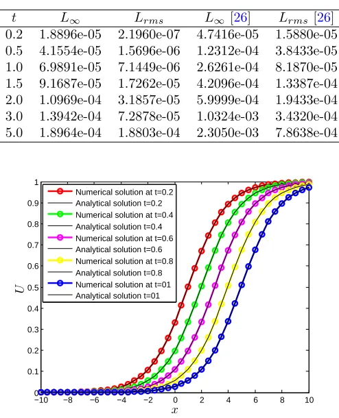
Test Problem 6. The exact solution [26] of the 1D nonlinear standard Fitzhugh-Nagumo
equa-tion (6) is
U(x, t) = 1
2 +
1
2tanh
1 2√2(x−
2ρ−1 √
2 t)
, x∈[−10,10] t≥0. (32)
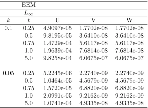
In Table8 we have calculated numerical results for Test Problem 6 with N = 101, dt= 0.0001
using MQ RBF. Table 8 shows Lrms and L∞ error norms of the EEM for q = 0.75. From the
table it can be seen that the obtained results are quite agreed with the results given in [26]. Fig.
1 shows the comparison of numerical and analytical solutions for t = 0.2,0.4,0.6,0.8,1, q = 4
and N = 41 for Test Problem 6 while Fig. 2 shows the numerical simulations of the EEM for
q= 0.75 and q= 4.
Test Problem 7. The exact solution [39] of 1D coupled KdV equation (7) withγ = 3 andα=β
is
U(x, t) = λ
αsech
2 1
2
r
λ
α(x−λt)
!
, V(x, t) =
q
1
αλsech2
1 2
q λ
α(x−λt)
√
2 .
Table 8: Comparison of FN equation using the EEM for Test Problem6.
t L∞ Lrms L∞[26] Lrms [26] 0.2 1.8896e-05 2.1960e-07 4.7416e-05 1.5880e-05 0.5 4.1554e-05 1.5696e-06 1.2312e-04 3.8433e-05 1.0 6.9891e-05 7.1449e-06 2.6261e-04 8.1870e-05 1.5 9.1687e-05 1.7262e-05 4.2096e-04 1.3387e-04 2.0 1.0969e-04 3.1857e-05 5.9999e-04 1.9433e-04 3.0 1.3942e-04 7.2878e-05 1.0324e-03 3.4320e-04 5.0 1.8964e-04 1.8803e-04 2.3050e-03 7.8638e-04
−10 −8 −6 −4 −2 0 2 4 6 8 10
0 0.1 0.2 0.3 0.4 0.5 0.6 0.7 0.8 0.9 1
x
U
Numerical solution at t=0.2 Analytical solution t=0.2 Numerical solution at t=0.4 Analytical solution t=0.4 Numerical solution at t=0.6 Analytical solution t=0.6 Numerical solution at t=0.8 Analytical solution t=0.8 Numerical solution at t=01 Analytical solution t=01
Figure 1: Comparing the curves of the numerical and analytical solutions forN = 41,q = 4 for
Test Problem6.
−10 −5
0 5
10
0 0.5
1 0 0.2 0.4 0.6 0.8 1
x t
U
−10 −5
0 5
10
0 0.5
1 0 0.2 0.4 0.6 0.8 1
x t
U
Figure 2: (Left) Numerical solutions for q = 0.75, (Right) Numerical solutions for q = 4 using
the EEM forN = 41, t= 1 for Test Problem 6.
In Table9, we have listed numerical simulations of the EEM versus results obtained from RBFs
based collocation method [39] for Test Problem7. The value of the parameters areα=β =λ=
Table 9: Numerical results of coupled KdV system in form of L2 error norm using the EEM for
Test Problem7.
t 0.1 0.2 0.3 0.4 0.5 1 2
[39]
U 3.662e-05 5.177e-05 4.065e-05 3.951e-05 3.964e-05 3.975e-05 4.461e-05 V 2.584e-06 3.648e-06 2.855e-06 2.769e-06 2.772e-06 2.749e-06 3.033e-06 EEM
U 8.3147e-08 3.3251e-07 7.4809e-07 1.3299e-06 2.0779e-06 8.3112e-06 3.3245e-05 V 5.8794e-09 2.3512e-08 5.2898e-08 9.4037e-08 1.4693e-07 5.8769e-07 2.3508e-06
Table 10: Numerical results of the EEM for Test Problem 8.
EEM
L∞
k t U V W
0.1 0.25 4.9097e-05 1.7702e-08 1.7702e-08 0.5 9.8195e-05 3.6410e-08 3.6410e-08 0.75 1.4729e-04 5.6117e-08 5.6117e-08 1.0 1.9639e-04 7.6814e-08 7.6814e-08 5.0 9.8258e-04 6.0675e-07 6.0675e-07
0.05 0.25 5.2245e-06 2.2740e-09 2.2740e-09 0.5 1.0464e-05 4.5679e-09 4.5679e-09 0.75 1.5720e-05 6.8820e-09 6.8820e-09 1.0 2.0991e-05 9.2162e-09 9.2162e-09 5.0 1.0741e-04 4.9335e-08 4.9335e-08
basis function withc= 100. From the listed results given in Table9, we have observed that the
results obtained by the EEM are better than the results given in [39].
Test Problem 8. The 1D Hirota-Satsuma coupled KdV system (8) with exact solution [28]
given below
U(x, t) = 4k2q2tanh2(ξ)−
8k2q2
3 −
C
3,
V(x, t) = 2k2q2tanh2(ξ)−
2k2q2
3 −
4 3 −c0,
W(x, t) = 2k2q2tanh2(ξ)−2k2q2+c0.
(34)
whereξ =√q2k(x−Ct) anda≤x≤b. In Table10the numerical simulations of Hirota-Satsuma
coupled KdV system (8) are carried out for Test problem8on the interval [−30,30] and different
values of kand t, with N = 13,dt= 0.05, using MQ RBF withc= 2. The value of parameters
C=c0 =q2= 0.1. A full agreement between numeric and exact solution have been observed.
Table 11: Comparison of numerical results of the EEM using GA RBF at point(0.40,0.60) for Test Problem9.
U V
t CPU time EEM [38] [46] Exact EEM [38] [46] Exact
0.30 0.17 0.3167 0.3168 0.3166 0.3166 3.1584 3.158 3.157 3.158 0.60 0.19 0.2726 0.2724 0.2725 0.2725 3.6696 3.669 3.667 3.669 0.90 0.23 0.2346 0.2347 0.2345 0.2346 4.2635 4.263 4.260 4.263 1.20 0.26 0.2019 0.2020 0.2018 0.2019 4.9534 4.953 4.950 4.953 1.50 0.30 0.1738 0.1739 0.1737 0.1738 5.7551 5.755 5.751 5.755 1.80 0.34 0.1496 0.1496 0.1495 0.1496 6.6864 6.686 6.681 6.686
a particular case in the region (x, y)∈[0,1]2,t≥0 with α= 1, β = 0,γ = 0.25 is given in [46]
U(x, y, t) = exp
−x−y− t 2
, V(x, y, t) = exp
x+y+ t 2
. (35)
The LMM is employed for the numerical solution of Test Problem9 by letting time step length
dt = 0.001, the shape parameter value c = 1, N = 20×20, at various times up to t= 1.8. In
Table11 we have compared the results obtained by the EEM with the exact solution as well as
with [38,46]. Reasonably good accuracy has been obtained in this case as well also CPU time in
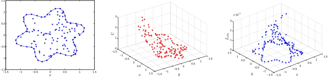
seconds are reported in the same table. The numerical results on irregular domains are shown in
Figs. 3-6for Test Problem9using MQ RBF with shape parameterc= 1. The numerical solutions
shown in Figs. 3-6are performed withdt= 0.001,t= 1α= 1,β= 0 andµ= 0.25. These figures
show the efficiency of the suggested method in irregular geometry in term of absolute errorLabs
by using the EEM for Test Problem9.
−1.5 −1 −0.5 0 0.5 1 1.5
−1.5 −1 −0.5 0 0.5 1 1.5
x
y
−1.5 −1
−0.5 0
0.5 1
1.5 −1.5
−1 −0.5
0
0.5 1
1.5 0
1 2 3
y x
U
−1.5 −1
−0.5 0
0.5 1
1.5
−1.5 −1 −0.5 0 0.5 1 1.5
0 1 2 3
x 10−3
x y
La
bs
Figure 3: Computational domain, numerical solution and absolute error by using the EEM for
−1.5 −1 −0.5 0 0.5 1 1.5 −1.5 −1 −0.5 0 0.5 1 x y −1.5 −1 −0.5 0 0.5 1
1.5 −1.5 −1
−0.5 0 0.5 1 1.5 0 1 2 3 y x U −1.5 −1 −0.5 0 0.5 1 1.5 −1.5 −1 −0.5 0 0.5 1 1.5 0 1 2 3 4
x 10−3
x y
La
bs
Figure 4: Computational domain, numerical solution and absolute error by using the EEM for
Test Problem9.
−1.5 −1 −0.5 0 0.5 1 1.5
−1.5 −1 −0.5 0 0.5 1 x y −1.5 −1 −0.5 0 0.5 1 1.5 −1.5 −1 −0.5 0 0.5 1 1.5 0 1 2 3 y x U −1.5 −1 −0.5 0 0.5 1 1.5 −1.5 −1 −0.5 0 0.5 1 1.5 0 1 2 3
x 10−3
x y
La
bs
Figure 5: Computational domain, numerical solution and absolute error by using the EEM for
Test Problem9.
−1.5 −1 −0.5 0 0.5 1 1.5
−1.5 −1 −0.5 0 0.5 1 1.5 x y −1.5 −1 −0.5 0 0.5 1
1.5 −1.5 −1
−0.5 0 0.5 1 1.5 0 1 2 3 y x U −1.5 −1 −0.5 0 0.5 1 1.5 −1.5 −1 −0.5 0 0.5 1 1.5 0 1 2 3
x 10−3
x y
La
bs
Figure 6: Computational domain, numerical solution and absolute error by using the EEM for
Test Problem9.
5
Conclusion
solutions available in the existence literature. On the basis of these results/ comparison we can conclude that the local meshless method is accurate, efficient and its implementation is very simple, straightforward, irrespective of the dimension and geometry of the problem.
Acknowledgements
This project was supported by the Theoretical and Computational Science (TaCS) Center under Computational and Applied Science for Smart Innovation Cluster (CLASSIC), Faculty of Science, KMUTT.
References
[1] S. Abbasbandy. Soliton solutions for the Fitzhugh-Nagumo equation with the homotopy
analysis method. Applied Mathematical Modelling, 32:2706–2714, 2008.
[2] G. Adomian. The diffusion Brusselator equation. Computers and Mathematics with
Appli-cations, 29:1–3, 1995.
[3] Imtiaz Ahmad, Siraj-ul-Islam, and Abdul Q. M. Khaliq. Local RBF method for
multi-dimensional partial differential equations. Computers and Mathematics with Applications,
74:292–324, 2017.
[4] A. M. Al-Rozbayani and M. O. Al-Amr. Discrete adomian decomposition method for solving
Burgers’-Huxley equation. International Journal of Contemporary Mathematical Sciences,
8:623–631, 2013.
[5] S. Ashrafi, M. Alineia, H. Kheiri, and G. Hojjati. Spectral collocation method for the
numerical solution of the Gardner and Huxley equations. International Journal of Nonlinear
Science, 18:71–77, 2014.
[6] L. M. B. Assas. Variational iteration method for solving coupled-KdV equations. Chaos,
Solitons and Fractals, 38:1225–1228, 2008.
[7] E. Babolian and J. Saeidian. Analytic approximate solutions to Burgers’, Fisher, Huxley
equations and two combined forms of these equations. Communications in Nonlinear Science
and Numerical Simulation, 14:1984–1992, 2009.
[8] H. O. Bakodah. Modified Adomain Decomposition Method for the generalized fifth order
KdV equations. American Journal of Computational Mathematics, 3:53–58, 2013.
[9] A. H. Bhrawy. A Jacobi-Gauss-Lobatto collocation method for solving generalized
Fitzhugh-Nagumo equation with time-dependent coefficients. Applied Mathematics and Computation,
222:255–264, 2013.
[10] M. Bukhari, M. Arshad, S. Batool, and S. M. Saqlain. Numerical solution of generalized
Burger’s-Huxley equation using local radial basis functions. International Journal of
Ad-vanced and Applied Sciences, 4(5):1–11, 2017.
[11] I. Celik. Haar wavelet method for solving generalized Burgers’-Huxley equation.Arab Journal
[12] M. T. Darvishia, S. Kheybari, and F. Khani. A numerical solution of the Lax’s 7th-order KdV
equation by Pseudospectral method and Darvishi’s preconditioning. International Journal
of Contemporary Mathematical Sciences, 2:1097–1106, 2007.
[13] K. Djidjeli, W. G. Price, E. H. Twizell, and Y. Wang. Numerical methods for the soltution
of the third and fifth-order disprsive Korteweg-de Vries equations. Journal of
Computation-aland Applied Mathematics, 58:307–336, 1995.
[14] S. M. El-Sayed and D. Kaya. An application of the ADM to seven-order Sawada-Kotara
equations. Applied Mathematics and Computation, 157:93–104, 2004.
[15] R. A. Fisher. The Wave of Advance of Advantageous Genes. Annals of Eugenics, 7:355–369,
1937.
[16] R. FitzHugh. Impulses and physiological states in theoretical models of nerve membrane.
Biophysical journal, 1:445–466, 1961.
[17] D. D. Ganji, M. Nourollahi, and M. Rostamian. A comparison of Variational Iteration
Method with Adomian’s Decomposition Method in some highly nonlinear equations.
Inter-national Journal of Science and Technology, 2:179–188, 2007.
[18] A. Goswami, J. Singh, and D. Kumar. Numerical simulation of fifth order KdV equations
occurring in magneto-acoustic waves. Ain Shams Engineering Journal, 2017.
[19] Sirajul Haq, A. Hussain, and M. Uddin. RBFs meshless method of lines for the numerical
solution of time-dependent nonlinear coupled partial differential equations. Applied
Mathe-matics, 2:414–423, 2011.
[20] G. Hariharan and K. Kannan. Haar wavelet method for solving Fitzhugh-Nagumo equation.
World Academy of Science, 43:560–564, 2010.
[21] M. A. Helal and M. S. Mehanna. A comparative study between two different methods for
solving the general Korteweg-de Vries equation (GKDV). Chaos, Solitons and Fractals,
33:725–739, 2007.
[22] R. Hirota and J. Satsuma. Soliton solutions of a coupled Kortewege-de Vries equation.
Physics Letters A, 85:407–418, 1981.
[23] A. L. Hodgkin and A. F. Huxley. A quantitative description of Ion currents and its
applica-tions to conduction and excitation in nerve membranes. Journal of Physiology, 117:500–544,
1952.
[24] H. N. A. Ismail, K. R. Raslan, and A. A. A. Rabboh. Adomian decomposition method
for Burgers’-Huxley and Burgers’-Fisher equations. Applied Mathematics and Computation,
159:291–301, 2004.
[25] M. Javidi. Modified pseudospectral method for generalized Burgers’-Fisher equation.
Inter-national Mathematical Forum, 32:1555–1564, 2006.
[26] Ram Jiwari, R. K. Gupta, and Vikas Kumar. Polynomial differential quadrature method for numerical solutions of the generalized Fitzhugh-Nagumo equation with time-dependent
[27] D. Kaya. An explicit and numerical solutions of some fifth-order KdV equation by
decom-position method. Applied Mathematics and Computation, 144:353–363, 2003.
[28] A. H. Khater, R. S. Temsah, and D. K. Callebaut. Numerical solutions for some coupled
non-linear evolution equations by using spectral collocation method.Mathematical and Computer
Modelling, 48:1237–1253, 2008.
[29] A. J. Khattak. A computational meshless method for the generalized Burgers’-Huxley
equa-tion. Applied Mathematical Modelling, 33:3718–3729, 2009.
[30] R. Lefever and G. Nicolis. Chemical instabilities and sustained oscillations. Journal of
Theoretical Biology, 30:267284, 1971.
[31] R. C. Mittal and A. Tripathi. Numerical solutions of generalized Burgers–Fisher and
gener-alized Burgers–Huxley equations using collocation of cubic B-splines. International Journal
of Computer Mathematics, 92(5):1053–1077, 2015.
[32] Mahdi Moghimia and Fatemeh S. A. Hejazi. Variational iteration method for solving
gener-alized Burgers’-Fisher and Burgers’ equations. Chaos, Solitons and Fractals, 33:1756–1761,
2007.
[33] J. S. Nagumo, S. Arimoto, and S. Yoshizawa. An active pulse transmission line simulating
nerve axon. Proceedings of the IRE, 50:2061–2070, 1962.
[34] Y. Pomeau, A. Ramani, and B. Grammaticos. Structural stability of the Korteweg-de Vries
solitons under a singular perturbation. Physica D, 31:127–134, 1988.
[35] J. Satsuma. Topics in soliton theory and exactly solvable nonlinear equations. World
Sci-entific, Singapore, 1987.
[36] Siraj-ul-Islam and Imtiaz Ahmad. A comparative analysis of local meshless formulation for
multi-asset option models. Engineering Analysis with Boundary Elements, 65:159–176, 2016.
[37] Siraj-ul-Islam and Imtiaz Ahmad. Local meshless method for PDEs arising from models of
wound healing. Applied Mathematical Modelling, 48:688–710, 2017.
[38] Siraj-ul-Islam, A. Ali, and Sirajul Haq. A computational modeling of the behavior of the
two-dimensional reaction-diffusion Brusselator system. Applied Mathematical Modelling,
34:3896–3909, 2010.
[39] Siraj-ul-Islam, Sirajul Haq, and Marjan Uddin. A meshfree interpolation method for the
nu-merical solution of the coupled nonlinear partial differential equations. Engineering Analysis
with Boundary Elements, 33:399–409, 2009.
[40] A. A. Soliman. A numerical simulation and explicit solutions of KdVBurgers’ and lax’s
seventh-order KdV equations. Chaos, Solitons and Fractals, 29:294–302, 2006.
[41] P. Thounthong, M. N. Khan, I. Hussain, I. Ahmad, and P. Kumam. Symmetric radial
basis function method for simulation of elliptic partial differential equations. Mathematics,
6(12):327, 2018.
[42] J. Tyson. Some further studies of nonlinear oscillations in chemical systems. The Journal
[43] M. Uddin and Siraj ul Haq. Application of a numerical method using radial basis functions
to nonlinear partial differential equations. Selcuk Journal of Applied Mathematics, 12:77–93,
2011.
[44] X. Y. Wang, Z. S. Zhu, and Y. K. Lu. Solitary wave solutions of the generalized
Burgers’-Huxley equation. Journal of Physics A: Mathematical and Theoretical, 23:271–274, 1990.
[45] A. M. Wazwaz. The decomposition method applied to systems of partial differential
equa-tions and to the reaction-diffusion Brusselator model. Applied Mathematics and
Computa-tion, 110:251–264, 2000.
[46] Ang Whye-Teong. The two-dimensional reaction-diffusion Brusselator system: a
dual-reciprocity boundary element solution. Engineering Analysis with Boundary Elements,
27:897–903, 2003.
[47] Y. T. Wu, X. G. Geng, X. B. Hu, and S. M. Zhu. Generalized Hirota-Satsuma coupled
Korteweg-de Vries equation and Miura transformations. Physics Letters A, 64:255–259,
1999.
[48] Y. Yamaoto and E. Takizawa. On a solution on non-linear time-evolution equation of
![table it can be seen that the obtained results are quite agreed with the results given in [∞26]](https://thumb-us.123doks.com/thumbv2/123dok_us/8011597.1331855/9.612.177.392.100.200/table-seen-obtained-results-quite-agreed-results-given.webp)