Normal Calculus on Moving Surfaces

(1)

Normal Calculus on Moving Surfaces

Keith C. Afas

†‡

University of Western Ontario

London, Ontario, N6A 5B7, CANADA

May 18th, 2018

Abstract

This paper presents an extension for principles of Differential Geometry on Surfaces (re-hashed through the budding field of CMS, the Calculus of Mov-ing Surfaces). It analyzes mostly 2D Hypersurfaces with Riemannian Ge-ometry and proposes the construction of a 3D Static Frame combining the Surface Basis Vectors with the Orthogonal Normal Field as a 3D Orthogonal Vector Frame. The paper introduces conventions for manipulating Tensors defined using this 3D Orthogonal Vector Frame as well as Curvature Connec-tions associated with this Vector Frame. It then finally introduces Symbols and Tensors to describe Inner Products and Variance within the 3D Vector Frame and then extends all the above concepts to a surface which is Dynamic utilizing principles from CMS. This formulation has potential to extend iden-tities and concepts from CMS and from Differential Geometry in a compact Tensorial Framework, which agrees with the new Framework proposed by CMS.

1 Introduction

1.1 Need For a new Calculus

(3)

especially paracellularly, involve events occuring on the surface of cells. [1, 19]

As expected from existing Physical Laws and Biochemical analyses of the membrane, the motions of the Cell Membrane are not exaggerated, but rather lethargic and appear to be periodic or at least bounded in some spa-tiotemporal nature [20, 21]. Methods to model this motion have yielded some, but still quite few analytical results — the bulk of which have been obtained over the past four decades [1, 2]. Most advances in this field of modelling have arose by modelling investigations which approximated Con-stitutive Equations of the Membrane and various Cytoskeletal components, and then proceeded apply various facets of Continuum Mechanics to the sur-face in an attempt to understand the effects of Microtubule Dynamics on the membrane [2, 3] and the effects of local Actin Concentrations to the surface [4].

Though these approaches are effective to an extent, much is left unan-swered that appear to be un-accountable for at the present. In some cases, unanswered questions arise due to the lack of extensive research in the field; in other important cases however, unanswered queries are due to the inher-ent limitations of the theoretical framework as it pertains to accounting for various interactions.

• The effects of shear stresses on the Membrane can be well approximated by the field of Continuum Mechanics, but accounting for any shear stresses by other cells with their own receptors cannot be well accounted for by the discipline

• It is already well understood that there exist cytoslic and extracellular interaction methods such as chemoattractants and various signalling pathyways that may change the Cell Membrane [1, 5, 6, 7], but the exact way to incorporate these into Continuum Mechanics is unclear.

• To this day, there, are little-to-none methods, to provide a direct An-alytic link between genetic regulation factors, and any aspects of the Central Dogma of Biology to their influence on Mechanical changes to the Membrane, though there is a very clear link [8, 9].

(4)

• Ultimately, there exists no theory which encompasses all the above in-teractions, and it is unclear what type of Mathematical theory would unite all the above, though it can be expected that such a theory would be intuitive, compact, easy to understand, geometric in nature, not be restricted to an ambient coordinate description, and capable of sup-porting theories sich as Field Theories, Biochemical interactions, and movements of Manifolds.

1.2 Existing Disciplines

The Need for Calculus

Right now, both the movements of Manifolds and Field Theories are united because they are described using the same language: Tensor Calculus.

Field Theories are described using Lagrangian Fields, Calculus of Vari-ations, and Classic Tensor Calculus, which are all summarized into Gauge Theories. These are important since they outline a compact way of describing all the already existing physical laws such as Electrodynamics and Quantum Field Theory in a compact and intuitive way [12].

The Movement of Manifolds over the years has had a few methods of description. Most recently, Movement of Manifolds was described by the new discipline of the Calculus of Moving Surfaces (CMS) which essentially describes a Geometric and Tensorial method of analyzing differential objects intrinsic and extrinsic to a manifold’s embedding [13], and introduces an operator which preserves the tensorial nature of Tensors under time differ-entiation [13, 18].

In reality, Lagrangian Mechanics, Hamiltonian, Newtonian, or Contin-uum Mechanics all provide ample methods of analyzing manifolds in their own respects, but can become ”unwieldy” when analyzing surfaces wholis-tically. CMS, though effective, lacks the application to solid 3D processes occurring within cells. Thus CMS could benefit from an investigation in attempting to alow it to acknowledge the 3D space it is embedded within before adressing 3D processes ocurring within cells.

(5)

con-struct a 3D Orthogonal Basis on a Surface unifying the Normal with the Surface Basis Vectors in an Orthogonal and Tensorial Fashion as the Surface deforms in time all in accordance with CMS.

2 An Intrinsic Surface Volumetric Dynamic

Coordinate Frame

2.1 Already Established Conventions

As a foreword, there are several conventions which will be used:

• CMS uses Einstein Summation Convention and draws on many of the conventions from Classical Tensor Calculus [13, 14, 15, 16]

• Different classes of indices imply different properties of tensors:

– Indices which refer to ambient space are denoted using Latin Char-acters (i,j,k,m,n,p,q); ie. in ambient space, the N-dimensional coordinate system is given by Zi _{= (}_Z1_{, Z}2_{, ..., Z}N_{) and the basis}

vectors with which the N-dimensional coordinate space that em-beds a surface is given by is denoted byZi and the ambient space’s

Metric Tensor which denotes distances in standardN-dimensional space is denoted by Zij.

– Indices which refer to the hypersurface’s (N −1) dimensional co-ordinate space are typically denoted using the first half of the Greek Alphabet. Here, the characters (α,β,γ,δ,,η,κ)will be used to denote surface components of tensors; ie. on the surface, the two-coordinate system required to specify its parameters are given by Sα _{= (}_S1_{, S}2_{, ..., S}N−1_{) and the surface’s tangent vector basis}

will be indicated by Sα, and the Surface Metric Tensor which

in-dicates distances across the surface are given by Sαβ)

– Indices which will be used to refer to the surface’s N-dimensional constructed coordinate space will be denoted using the second half of the Greek Alphabet. Here, we will use (µ,ν,λ,σ,ω,ζ,φ) to denote the components of a Dynamic Frame Tensor. ie. in this recon-structed space, it will posess the coordinates ξµ = (ξ1, ξ2, ..., ξN) and the basis in this coordinate frame will be given by ξ_µ)

(6)

• Apostrophes on an index imply a different coordinate change, and are related to the un-apostrophed coordinate systems by Jacobians. In transforming from one coordinate system to another, several different jacobians will be thrown into usage identifiable by the class of index they are using:

– In transforming from one ambient coordinate system to another, we will follow the convention that:

∂Zi₍_Z0₎

∂Zi0 =J i

i0 (1)

– In transforming from one surface coordinate system to another, we will require two jacobians. This is because the transformation does not just depend on the new coordinate system, but also depends on time because the surface is in motion.

∂Sα(t, S0)

∂Sα0 =J α

α0 ,

∂Sα(t, S0)

∂t =J

α

t (2)

These all have inverses associated for them and upon each’s mul-tiplication with its respective inverse, you produce the Kronecker Delta of the systems:

J_ii0Ji 0

j =δ

i

j , J

α α0Jα

0

β =δ

α

β (3)

• At times, tensors can have relevance to more than one coordinate sys-tem, and they do not necessarily require to be explicitly dependent on both of the coordinates. For example, Zi_α(t, S)

• There are several tensors which already have already been reserved for describing surfaces [13, 14, 15, 16]:

– The Position Tensor, R(t, S) =Zi₍_{t, S}₎_Z

i : This tensor describes

the position of every point of the surface.

– The Ambient Velocity, V = ∂tR = ViZi : This object can be

proven to not transform like a tensor, but is still of crucial impor-tance to describing the movement of the surface and much like the Christoffel Symbols, combine with other objects to form a tensor.

– The Shift Tensor,Zi

α =∇αZi : This tensor is an explicit relation

between the surface and the ambient space. It has the property that multiplying it by either the Surface Basis Vectors or the Am-bient Vectors can produce the opposite basis (Zi

αZi =Sα, ZiαS

α₌

(7)

– The Surfacial Levi Civita Symbols, αβ : This completely

anti-symmetric tensor is a representation of the permutation algebra which is inherent in the cross product and in the definition of antisymmetric tensorial components.

– The Normal, N=NiZi. The Normal is an essential tensor which

describes the direction that is projected ‘outwards’ infinitesimally from each tangent space. It is of crucial importance in defining ob-jects such as curvature and also is explicitly constructable from the shift tensor according to the following formula:Ni = 1₂ijkαβZαjZβk.

– The Surface Metric Tensor,Sαβ =Sα·Sβ : This symmetric tensor

follows from analogue from the standard metric tensor of space and describes the cooefficients required to measure distances along the surface. Much like the Ambient metric tensor, it can be used to define Christoffel Symbols of its own and is crucial when specifying Laplacians on the surface

– The Surface Christoffel Symbols, Γγ_αβ : Like the Ambient Christof-fel Symbols, this object is not a tensor, but can be used to create the definition of the Covariant Derivative, ∇α which operates on

various ambient and surface tensors and can also be constructed explicitly from the Surface Metric Tensor in a similar fashion as the Ambient Christoffel Symbols can be constructed from the Am-bient Metric Tensor.

– The Normal Velocity, C = V·N : This is an invariant tensor quantity constructed from a tensor and non-tensor, and intuitively describes the surface’s speed in the normal direction. In addition, it can also be seen in a Vector form which is defined asC=CN= (V·N)N.

– The Surface Velocity,Vα =V·Sα: This object is not a tensor, but like the Christoffel Symbols, is of essential importance to defining the tensorial operator which captures time differentiation in an invariant way.

– The Curvature Tensor,Bαβ =N· ∇αSβ =−Sβ· ∇αN: This

sym-metric tensor is one of the most important tensors in describing Static & Dynamic Surfaces. This tensor can be used to obtain the Mean and Gaussian Curvature of the surface. As a general rule, its trace is twice the surfaces mean curvature, and its determinant is the surface’s Gaussian Curvature. It also satisfies many inter-esting equivalencies such as the Codazzi Equation (∇[αBβ]γ = 0)

(8)

– The Surface Riemann Curvature Tensor,Rγ_δαβ = 2(Γγ_δ_[_β,α_]+Γγ_[_αΓ_β_]_δ) = 2B_[γ_αBβ]δ : This Tensor is an Surfacial analogue of the Riemann

Curvature Tensor which describes the curvature of space and is determined from the antisymmetric components of the Christoffel or Curvature Tensors. This is crucial for defining Ricci Curvature on the Surface.

– The Tensorial Time Derivative, ˙∇ : Much like the Covariant Derivative, this Derivative’s form changes depending on the Ten-sor it is acting on. This operator is an effective method to capture infinitesimal change of a Dynamic Field defined on a surface in the normal direction, and therefore is invariant under changes to the surface coordinates. This makes it a critical operator. For invari-ant fields, the derivative assumes the form: ˙∇ψ = ˙ψ−Vα_∇

αψ.

– The Temporal Symbols, ˙Γα

β =∇βVα−CBβα : These symbols are

not Tensors by no means, but effectively assume the role in the Tensorial Time Derivative of Surface Tensors that the Christoffel Symbols play in the Covariant Derivative

– The Temporal Curvature Tensor, ˙Rγ_αβ = 2SγδBα[β∇δ]C : This

Tensor Describes the commutation between the Covariant Deriva-tive and the Tensorial Time DerivaDeriva-tive acting on a Surface Vector [18].

2.2 Creating the Static Frame

Letting ΣS be the set of all possible deformed surfaces from an original

surface, S. For all surfaces, and more specifically - for the subset of surfaces that can be classified as isosurfaces for all cells, BS ⊂ ΣS - the surfaces

possess intrinsically two Surface Basis Tensors, Sα. For these two surface

tensors a third tensor is defined which is orthogonal to the other two surface tensors. This tensor is commonly known as the Normal (of unit length) and is explicitly given by [14]:

N=S1×S2 (4)

This may be formulated into a component by component form [13]:

N= 1 2Z

i

ijkαβZjαZ

k

β (5)

This is critical for the definition of the coordinate frame. The collection of the Vectors {S1,S2,N} is referred to as the Static Frame and is extremely

(9)

has an intrinsically geometric significance. It is exactly the local euclidean space which is rotated to be tangent with the surface locally. To highlight this, considering the flat Surface described parametrically by z(x, y) = 0. It can be intuitively seen that its two Surface Basis Vectors are in fact ˆi & ˆj. In addition, the normal can be explicitly derived to reveal the intuitive notion that its normal is given by N = ˆk. Thus the collection of the Static Frame Vectors can be identified as {ˆi,ˆj,ˆk} which highlights the relationship of the static frame in relation to the Local Euclidean Basis.

For every surface, it will have its own intrinsic static frame. This frame is assumed to be composed of a curvilinear varying basis, denoted by ξ_µ. As a general formality, the Shift Kronecker Tensor is introduced ˜δα

µ. to relate

the surface indices with the Static Frame’s indices. If the local coordinate space is considered within the Static Frame, along with the geometric na-ture of the surface that the Static Frame is embedded upon, the three basis vectors which define this frame can be explicitly stated:

ξ_µ={S1,S2,N} (6)

Using this basis, any tensor from a surface’s apex may be defined. Suppose

T is a tensor. In terms of the local coordinate basis, this may be expressed as:

T=Tµξ_µ =TαSα+T3N (7)

The interesting aspect of this decomposition is the reduction for a covariant tensor:

T=Tµξµ =TαSα+T3N (8)

Most interestingly, it seems that the decomposition implies the following universal equality: T3 = T3. This is due to the fact that for basis vectors,

their dual is defined from the geometric condition that regarding the aspect of magnitude, they must be unit vectors (ie. S1 ·S1 = 1,S2 ·S2 = 1). This

holds water with the first two basis vectors and even has the Kronecker Delta defined from their multplication: Sα·Sβ =δβα. However, the Normal cannot

be continued from the definition; this is because although it is orthogonal to the other basis vectors, it is not defined independently of the Surface Basis Vectors as highlighted by Eq.(4). The definition of the Normal is exactly from the algebraic product of the Surface Basis Vectors, and thus cannot have the index exteded to to being the ‘Third’ Surface Basis Vector. In fact, it is completely orthogonal to the other basis vectors:

Sα·N= 0→(ξµ·ξ

3

(10)

Therefore, in order to rectify its independence from the surface basis vectors, it actually is its own dual. Without specifying any indices (making it a Tensor of Rank 0, with Rank-1-components), it is its own dual:

N·N= 1 →ξ₃·ξ3 = 1 (10) Therefore, any tensor components associated to the Normal Basis vectors will have no distinction between being ‘Contravariant or Covariant. They simply are independent Scalar Fields who have an arbitrarily Raised/Lowered index for the purposes of a placeholder. This is illustrated when the Metric Tensor is obtained later on.

A Notation for the Static Frame

The Static Frame uses Tensors with the indices (µ,ν,λ,σ,ω,ζ,φ). Whenever a static frame index is noted, it will run from, 1..N. The problem with that is that since it is a N- Vector Space constructed from a Manifold of (N-1) Dimension, the N index values can actually be classified into two sets. The first (N-1) index values needed for the surface parametrization, and the Nth index value which actually represents the Normal Direction. Therefore, when representing a vector for example, the first (N-1) entries are all presided over by CMS, and the Nth Entry corresponds to the last entry directly linked to the static frame. For this reason, suppose a (N=28) dimension Static Frame is being observed. The first 27 index values are all abbreviated as the surface indices.

Therefore for example; a Vector may be represented within a 28 di-mension Static Frame as a 2-entry Vector. One entry representing the 27 surface entries and the second entry for the Normal Representation. For example if the Vector on the surface was given in _R3_{, on a hypersurface of}

dimension of 2:

V=V1S1+V2S2+V3N

Using the conventions of CMS, this can be abbreviated into a surface com-ponent and a Normal Comcom-ponent:

V =Vµξ_µ =VαSα+V3N

Therefore, in abrreviating vectors in this space with respect to the bases, it can be represented in the following manner:

Vµ=

Vα

V3

(11)

A Matrix may be constructed on the surface in the following manner: If it has components given by

¯

V =Vµν(ξ_µ⊗ξ_ν) = Vαβ(Sα⊗Sβ)+Vα3(Sα⊗N)+V3β(N⊗Sβ)+V33(N⊗N)

Then it can be represented as:

Vµν =

Vαβ _Vα3

V3β _V33

(12)

This convention will be largely for notating Vectors And Matrices in the Static Frame.

2.3 The Frame Coordinates & the Normal Coordinate

Unlike other analyses of space, here there is use for the coordinates to be obtained after the basis vectors have been defined. In following with the general convention, the two coordinates, Sα _{which are parallel to the surface}

basis vectors are identified in the following manner [13]:

∂R

∂Sα =Sα (13)

Issues arise when attempting to identify the same analogy with the Normal. With the Normal, there is no logical coordinate that one might use to define the ‘direction’ of the Normal since the manifold is of (N −1) dimensions. By analogy, the Normal Derivative might be defined as the partial derivative which goes infinitesimally in the general direction of this new informal ‘Nor-mal Coordinate’ denoted as n; the identity of this derivative as a directional derivative will become more obvious momentarily. As expected, the action of this partial derivative on the Position Vector yields the Normal [15]:

∂R

∂n =N (14)

However, we already know that the normal can also be expressed in its coor-dinate form asN=Ni_Z

i, and the ambient basis is just the partial derivative

of the position vector in each of the ambient coordinates, (Z1_{, Z}2_{, Z}3_{). Since}

the position vector is an invariant tensor of rank zero, we can also express its partial derivative as its covariant derivative. Thus we can also express the above as the following equivalency:

∂R

∂n =N

i_Z

i →

∂R

∂n =N

i_∇

iR→

∂ ∂n−N

i_∇

i

(12)

In this equation, the definition of the normal coordinate is given in a differ-ential form. This is the theoretical properties of the coordinate’s derivative. We also directly obtain the normal derivative. This is given as:

∂

∂n = (N· ∇) (16)

Searching for a rigourous definition of the coordinate, we see that the follow-ing equality should hold:

∂

∂nn= 1 = (N· ∇)n (17)

Since we know that the Normal is a unit vector, then we see that the normal coordinate is the ambient scalar field which satisfies the following equation:

∇n =N (18)

Therefore, we see that there is no exact definition of the normal coordinate yet, but it still satisfies very real differential properties, and thus has an existence.

2.4 Change of Coordinates

If we allow the frame to change (such as a change of surface coordinates, we see that to maintain an invariant tensor, we have the following difference

T0 =Tµ0ξ_µ0 =Tµ 0

˜

J_µµ0ξ_µ=Tα 0

˜

J_αα0S_α+T3 0

˜

J₃α0S_α+Tα 0

˜

J_α30N+T3 0

˜

J₃30N (19)

However from the linear nature of the tensor, we know that the form of the tensor under transformation must be as following:

T0 =Tµ0ξ_µ0 =Tα 0

Sα0 +T3 0

N=Tα0J_αα0S_α+T3 0

N (20)

Therefore, we see that by equating the two equations, the form of a jacobian must be of the following:

J_µµ0 =

Jα

α0 0

0 1

(21)

(13)

3 Differential Connections in the Static Frame

3.1 Distances Measured in the Static Frame

Much like the ambient space, the Static Frame’s 3d space has a Metric Which denoted distance along its coordinates. We allow this metric to be denoted by ξµν. Much as in the Surface Metric Tensor and as in the Ambient Metric

Tensor, we define the Metric in the Static Frame to be:

ξµν =ξµ·ξν (22)

Since this has a particular form in the case that either of the indices are 1 & 2, or 3, there will be 4 distinct components for the Metric Tensor which should be symmetric. We find that the 4 cases are well summarized as the following table:

˜

δµ

αδ˜νβξµν =Sαβ δ˜µαξµ3 = 0

˜

δµ_βξ3µ = 0 ξ33 = 1

(23)

This Metric can be well summarized in the following Matrix Form:

ξµν =

Sαβ 0

0 1

(24)

For such a metric, we can say that the length of any infinitesimal distances in this space are given by:

ds2 =SαβdSαdSβ+dn2 (25)

And the dot product of any two vectors, A and B, in this space is given by the following:

A·B=AµBµ =ξµνAµBν =SαβAαBβ +A3B3 (26)

(14)

verified algebraically by the following:

|ξµν|=

1 3!e

µνλ_eσωυ_ξ

µσξνωξλυ

|ξµν|=

1 3!e

µνα_eσωβ_ξ

µσξνωSαβ +

1 3!e

µν3_eσω3_ξ

µσξνω

|ξµν|=

1 3!e

3γα_e3δβ_S

γδSαβ +

1 3!e

γ3α_eδ3β_S

γδSαβ +

1 3!e

αβ3_eγδ3_S

αγSβδ

|ξµν|=

1 3!e

γα_eδβ_S

γδSαβ +

1 3!e

γα_eδβ_S

γδSαβ+

1 3!e

αβ_eγδ_S

αγSβδ

|ξµν|=

1 3!e

γα_eδβ_S

γδSαβ +

1 3!e

γα_eδβ_S

γδSαβ+

1 3!e

γα_eδβ_S

γδSαβ

|ξµν|=

3 3!e

γα_eδβ_S

γδSαβ

|ξµν|=

1 2!e

γα_eδβ_S

γδSαβ

|ξµν|=|Sαβ|

We also define an interaction between the Static Frame and the Ambient Coordinate Frame; we define this as the Twist Tensor. This is given by:

ζi_µ=Zi ·ξ_µ (27)

The Twist Tensor is realized as the following matrix:

ζi_µZi⊗ξµ=





Z1

1 Z12 N1

Z2₁ Z2₂ N2 Z3

1 Z32 N3 

 (28)

Or the equivalent:

ζi_µ=

Zi

α Ni

(15)

We can semi-use the definition of the determinant [13] to derive the property of the Twist Tensor:

|ζi_µ|= 1 3!eijke

µνλ_ζi

µζ

j

νζ

k λ

|ζi_µ|= 1 3!eijke

µνα_ζi

µζ j νZ k α+ 1 3!eijke

µν3_ζi

µζ

j

νN

k

|ζi_µ|= 1 3!eijke

µβα_ζi

µZ j βZ k α+ 1 3!eijke

µ3α_ζi

µN

j_Zk

α+

1 3!eijke

µν3_ζi

µζ

j

νN

k

|ζi_µ|= 1 3!eijke

3βα_Ni_Zj

βZ

k

α+

1 3!eijke

β3α_Zi

βN

j_Zk

α+

1 3!eijke

αβ3_Zi

αZ

j

βN

k

|ζi_µ|= 1 3!eijke

βα3_Zj

βZ

k

αN

i₊ 1

3!ejike

βα3_Zi

βZ

k

αN

j ₊ 1

3!ekije

αβ3_Zi

αZ

j

βN

k

|ζi_µ|= 1 3

1 2!eijke

βα

Zj_βZk_α

Ni+ 1 3

1 2!ejike

βα

Zi_βZk_α

Nj +1 3

1 2!ekije

αβ

Zi_αZj_β

Nk

|ζi_µ|= 1 3

p |Sαβ|

p |Zij|

1 2!ijk

βα_Zj

βZ

k α

Ni+

1 2!jik

βα_Zi

βZkα

Nj+

1 2!kij

αβ_Zi

αZ j β Nk

|ζi_µ|= 1 3

p |Sαβ|

p |Zij|

(NiNi+NjNj +NkNk) =

p |Sαβ|

p |Zij|

=

r

S Z

3.2 Surface Variance in the Surface Basis Vectors

At this point it is appropiate to analyze how the Basis Varies from point to point. We may begin by first analyzing the definition of the Christoffel Symbols in terms of the Surface Vector’s partial derivatives:

Γγ_αβ =Sγ· ∂Sα

∂Sβ (30)

Any variance of the surface vectors in the direction of the Normal is referred to the Curvature Tensor, this is delineated by:

Bαβ =N·

∂Sα

∂Sβ (31)

As we would expect, applying the definition of the Covariant Derivative to the Surface Vector’s partial derivative, and also using the known definition of the Surface Vector’s covariant derivative, ∇βSα =NBβα we see the following

expected identity arise:

∂Sα

∂Sβ =∇βSα+ Γ γ

(16)

This identity agrees with the two observations in the above two equations. We can also abbreviate this using the Static Frame’s basis:

∂Sα

∂Sβ = Γ µ

αβξµ (33)

Where the Christoffel Symbols of the Static Frame will be discussed in more detail.

3.3 Normal Variance in the Basis Vectors

We see that in general, it is very difficult to define the Normal Derivative on Surface Differential Objects. Here we use the φ,i notation to indicate the

partial derivative of φ. We know that for a 3d ambient coordinate system, for a spatiotemporal ambient field, φ(t, Z) the following identity holds [17]:

φ,[ij]= 0 (34)

Normally for a surface coordinate system, we also see that for a spatiotem-poral field, ψ(t, S) the following identity holds [16]:

ψ,[αβ]= 0 (35)

Motivated by the following two examples, we state a requirement of our coor-dinate system; for a field defined in the region of a surface in the Static Frame, Ω(ξ), we state that the coordinate’s partial derivatives must commute:

Ω,[µν]= 0 (36)

As we can see by the above examples, this holds for the Surface Coordi-nate Partial Derivatives, but is left ambiguous by the Normal Derivative. Following from the above requirement, we state the resultant commutation condition that:

∂ ∂n,

∂ ∂Sα

Ω = 0 (37)

3.4 A more General Normal Derivative

Thus, we then re-define a normal derivative which manifests more generally than the other definition. We first state that this derivative must satisfy the following requirements:

∂φ ∂n =

∂φ ∂ξ3 ,

∂R

(17)

We can utilize this derivative antisymmetric relation to obtain all sorts of relations within CMS. If we apply the last condition to the position vector:

∂ ∂n,

∂ ∂Sα

R= 0→ ∂Sα

∂n =∇αN (39)

The following fundamental identity forms:

∂Sα

∂n =−B

β

αSβ (40)

As expected, the normal derivative of the tangent vectors, too, lies in the tangent plane [13]. This also extends to the Surface Metric Tensor, and using the relation SαβSβγ = δγα can also be extended to the inverse Metric

Tensor:

∂Sαβ

∂n =−2Bαβ ,

∂Sαβ

∂n = 2B

αβ ₍₄₁₎

Therefore, based on the symmetry of the Inverse Metric Tensor, there exists a Normal Derivative on the contravariant Metric Tensor:

∂Sα

∂n =B

α

βS

β

(42)

It can be automatically seen that the new Normal Derivative preserves the Tensorial Identity of its Tensors that it operates on by assuming the Com-mutation of the Frame’s partial derivatives. Allowing the Normal Derivative of the Normal to be assumed as the following form:

∂N

∂n =K

µ_ξ

µ

By applying the Normal Derivative to two Normal Vector identities, we can specify the exact form of the Derivative. First by applying the Normal Derivative to both sides of the equation of its unit length conditionN·N= 1, and assuming the theNormal Derivative satisfies the Liebniz Product Rule, then we see that:

N· ∂N

∂n = 0

Also by considering its orthogonality with the Tangent Vectors and Normal Differentiating both sides of the equation N·Sα = 0, the following identity

also arises:

∂N

∂n ·Sα = 0

Therefore, we see that the only way to rectify these two conditions is if we establish the fundamental result:

∂N

(18)

This fundamental result arises as expected: this is because since the normal is in the direction of the normal derivative, it should have no variation in that direction. Both of the fundamental identities arise because of the assumption that this new Normal Derivative must commute with the Surface Partial Derivatives.

3.5 Extending the Surface-Normal Commutator

If we apply the commutation to the invariant field that is the Normal, we see that:

∂

∂n(∇αN) =0→ ∂ ∂n(B

β

αSβ) =0 (44)

This can be utilized to obtain the following relation:

∂Bβ α

∂n =τ

β

α (45)

This can be used to obtain the similar relation to the other forms of the Curvature Tensor and We finally see that:

∂Bαβ ∂n = 3τ

αβ _, ∂B

β α

∂n =τ

β

α ,

∂Bαβ

∂n =−ταβ (46)

In addition, we can apply the commutator to the Tangent Vectors and we obtain the following relation:

∂ ∂n, ∂ ∂Sα Sβ =

∂ ∂n Γ

γ

αβSγ+BαβN

+ ∂

∂Sα B γ

βSγ

∂ ∂n, ∂ ∂Sα

Sβ =Sγ

∂ ∂nΓ γ αβ−Γ γ αβB δ

γSδ+

∂Bαβ

∂n N+ ∂Bγ_β

∂SαSγ+B γ

β Γ

δ

αγSδ+BαγN

∂ ∂n, ∂ ∂Sα

Sβ =Sγ

∂ ∂nΓ

γ

αβ+Sγ∇αBβγ

Assuming that the Commutation Vanishes, we see that:

∂ ∂nΓ

γ

αβ =−∇αB

γ

β (47)

We can use this to find how the Riemann Curvature Tensor of the Surface Varies in the Normal Direction. For example, if we define the Riemann Curvature Tensor on the Surface as [13]:

(19)

And seeing that we know the normal derivative of the Christoffel Symbols, we can definitively define the Normal Derivative of both sides of the Equation

∂ ∂nR γ δαβ = ∂ ∂n

2Γγ_δ_[_β,α_]+ 2Γ_δ_[_βΓγ_α_]

∂ ∂nR

γ

δαβ = 2

∂ ∂nΓ

γ

δ[β,α]+ 2Γ

δ[β

∂ ∂nΓ

γ

α]+ 2Γ

γ [α ∂ ∂nΓ β]δ ∂ ∂nR γ

δαβ =−2

∇δB

γ

[β

,α]−2Γ

δ[β∇α]Bγ−2Γ

γ

[α∇β]B

δ

Here we see that we can turn the first term into a Covariant Derivative form and Insert the Chrisoffel Symbols obtained by this conversion into Covariant Derivative format. Here we know that: ∇δB

γ β

,α=∇α∇δB

γ

β + Γ

αβ∇δBγ +

Γ

αδ∇Bβγ−Γγα∇δBβ. Since there is a commutation on all the terms, and by

the symmetry of the Christoffel Symbols, we know that the second term will vanish and using the Codazzi Equation [14, 16], we are left with the following result:

∂ ∂nR

γ

δαβ =−2

∇[α∇β]Bγ_δ −Γγ_[_α∇β]Bδ+ Γ

δ[α∇β]Bγ

−2Γ_δ_[_β∇α]Bγ−2Γ γ

[α∇β]B

δ

From here we see that the second and last terms will cancel out, and because the third terms and fourth terms are symmetric, they will vanish under the commutation. Therefore we are left with the following equation:

∂ ∂nR

γ

δαβ =−2∇[α∇β]Bδγ

And we can utilize the definition of the Riemann Curvature Tensor to finally obtain the following:

∂ ∂nR

γ

δαβ =R

δαβBγ−R

γ

αβB

δ (48)

This formula can also be put into an Eigen-operator form:

∂ ∂nR γ δαβ = (δ η δB γ −δ γ B η

δ)R

ηαβ (49)

While this operator may seem not useful to use at first, it actually can be used to obtain serveral relationships. For example, using this we can obtain the Normal Derivative of the Ricci Tensor by contracting the Two Indices required using the Kronecker Delta:

∂

∂nRδβ = (δ

η δB α −δ α B η

δ)R

ηαβ =B

α

R

ηαβ−RηβBδη (50)

We can also obtain the Normal Derivative of the Ricci Curvature by con-tracting the equation with the Metric Tensor:

∂Rα α

∂n = 2R

α

βB

(20)

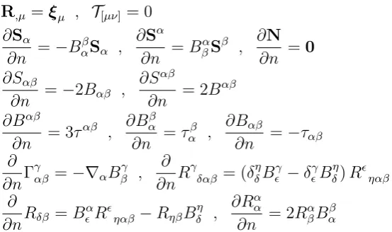
3.6 Table of Normal Derivatives of Static Objects

Here we have obtained several relationships on the objects defined on a sur-face and will concisely state them here:

R,µ =ξµ , T[µν]= 0

∂Sα

∂n =−B

β

αSα ,

∂Sα

∂n =B

α

βS

β

, ∂N ∂n =0 ∂Sαβ

∂n =−2Bαβ ,

∂Sαβ ∂n = 2B

αβ

∂Bαβ

∂n = 3τ

αβ _, ∂Bαβ

∂n =τ

β

α ,

∂Bαβ

∂n =−ταβ ∂

∂nΓ

γ

αβ =−∇αBβγ ,

∂ ∂nR γ δαβ = (δ η δB γ −δ γ B η

δ)R

ηαβ

∂

∂nRδβ =B

α

Rηαβ−RηβB

η

δ ,

∂Rα_α ∂n = 2R

α βBαβ

4 Covariant Derivatives in the Static Frame

4.1 Formulating a Covariant Derivative

It is at this point that we consider the covariant derivatives of the coordinate frame. We begin by establishing that for a invariant tensor, T, its Static Frame Covariant Derivative, ˜∇µ will be defined by:

˜

∇µT=

∂T

∂ξµ (51)

If we assume thatTis of the formT=Tµ_ξ

µ(ie. it is a contravariant tensor),

then we can simplify the expression further:

˜

∇µT=

∂Tν

∂ξµξν+T

ν∂ξν

∂ξµ

The second term of the equation has benefit if it is separated into its Normal and Surface Components due to the partial derivative of the basis vectors becoming more clear:

˜

∇µT=

∂Tν

∂ξµξν+T

α∂Sα

∂ξµ +T

3∂N

∂ξµ

Since we know how the Basis Frame behaves under the Normal Derivative, then in the special case that µ= 3 the Covariant Derivative reduces to:

˜

∇3T=

∂Tν

∂n ξν +T

ν∂ξν

∂n = ∂Tν

∂n ξν −SαB

α

βT

(21)

The other case where the indices are in fact Surface Indices are more complex. We see that we can expand the partial derivatives of the Basis Vectors to obtain:

˜

∇βT=

∂Tν

∂Sβξν +T

α₍_N_B

αβ + ΓγαβSγ)−T3SγBβγ (53)

4.2 The Frame Christoffel Symbols

All the terms can be grouped together if an object denoted as the Frame Christoffel Symbols are defined by:

˜ Γν_βµ =

Γα

βγ −Bβα

Bβγ 0

, Γ˜ν₃_µ=

−Bα

γ 0

0 0

(54)

Much like the other Christoffel Symbols, these are Symmetrical in Nature:

˜

Γν_µσ = ˜Γν_σµ (55)

Using the definition of the Frame Christoffel Symbols, the Covariant Deriva-tive can be summarized in the form as:

˜

∇βT=

∂Tν ∂Sβ + ˜Γ

ν

βσTσ

ξ_ν (56)

In fact, if we use the definition of ˜Γµ₃_σ, then

˜

∇µT=

∂Tν

∂ξµ + ˜Γ ν

µσT

σ

ξ_ν (57)

4.3 The Frame Covariant Derivative & Metrilinic

Prop-erties

Now, noticing that the Covariant Derivative must obey the Liebniz Product Rule on an invariant, we obtain the following identity:

˜

∇µTν =

∂Tν

∂ξµ + ˜Γ ν

µσT

σ ₍₅₈₎

This Covariant Derivative does not seem different from the ones given in standard literature. However, this also implies a very crucial identity about the Covariant Derivative we have formed. We also notice that the following identity is going to hold:

˜

(22)

The beautiy of this equation is that as expected, it follows all the conventions as you would expect in a covariant derivative. For any three dimensional ambient space, we know that:∇iZj = 0; this reaffirms the central concept

that the Static Frame is as good of a basis vector frame as any other ambient space coordinate system. When applied to a covariant tensor, it has the following form:

˜

∇µTν =

∂Tν

∂ξµ −Γ˜ σ

µνTσ (60)

The Frame Christoffel Symbols play a very interesting role in defining a new Calculus on the Basis Vectors. There is a very crucial difference between the Surface Covariant Derivative and the Surface Projection of the Static Frame Covariant Derivative; this can be concisely summarized as: ˜∇αSβ 6=

∇αSβ. We see expanding the covariant form of the Static Frame Covariant

Derivative:

˜

∇αSβ =

∂Sβ

∂Sα −Γ˜ σ

αβξσ =

∂Sβ

∂Sα −Γ˜ γ

αβSγ−Γ˜

3

αβN

After expanding the definition of the partial derivative of the Surface Vectors, then we see that the covariant derivatives vanish; this of course is different than the Surface Covariant Derivative of the Surface Vectors, because as it is already known: ∇αSβ =NBαβ. This is accomplished entierely by the unique

new Frame Christoffel Symbols.As a general rule we see that in general when acting on Tensors of Rank greater than (0,0), then the following identity holds:

˜

∇α 6=∇α (61)

For a Contravariant Tensor of rank (1,0) embedded in the Frame SpaceT=

Tµ_ξ

µ, we see that by expanding the Frame Christoffel Symbols, we can obtain

the following for the Tensor’s Surface Components:

˜

∇βTα=∇βTα−BβαT

3

(62)

For a Covariant Tensor, then we see that for the Surface Components:

˜

∇βTα =∇βTα−BαβT3 (63)

We see that we can also use the equation to find the Divergence in the Static Frame of a Frame Tensor. This is given on an Invariant Tensor in the Frame by:

˜

(23)

4.4 Local Curvature of the Static Frame Space

We notice that when analyzing the Commutation of the Static Frame’s Co-variant Derivatives, we should have the following identity:

2∇[µ∇ν]ψ = 0 (65)

However, what does occur us that when the commutation is applied to a Static Frame Tensor, the folliwing identity forms itself:

2∇[µ∇ν]ψσ = ˜Rσλµνψ

λ ₍₆₆₎

Where ˜Rσ_λµν has the same definition as the regular Curvature Tensor:

˜

Rσ_λµν = 2(˜Γσ_λ_[_ν),ν]+ 2˜Γσω[µΓ˜ ω

ν]λ (67)

If we calculate the curvature’s 81 components, using the following identity:

∂

∂nBαβ =−ταβ (68)

Then the stunning result follows:

˜

Rσ_λµν = 0 (69)

This is interestingly strong result; It is seen that the Christoffel Symbols are definitely non-zero, and depend on the structure of the Surface, but however based on the organization of the Coordinate System, the whole Riemann Curvature Tensor Vanishes. This means that the Static Frame Covariant Derivatives Vanish commute with a tensor. Therefore we also can state that for the 3 dimensional space in the neighbourhood of a Surface:

˜

Rµν = ˜Rσµσν = 0,R˜=ξ µν_R_˜

µν = 0 (70)

5 The Dynamic Frame

We now move on an essential and grand generalization; Normally, our surface will depend on time. In the case that the surface is moving, the calculus which is formed upon tensors changes. In fact, we see that now, the frame which was assumed to be static is now in fact dynamic. Therefore we proceed to state the Dynamic Frame’s Coordinates:

(24)

5.1 Invariant Theta Symbols

Using certain elements from the Extension of CMS [13], we see that we can express the Invariant Time Derivatives of all the Basis Vectors. If we recall the following Elements from the Extension of CMS:

˙

∇Sα = (∇αC)N , ∇N˙ = (−∇αC)Sα

We can therefore abbreviate this in a symbol:

˙

∇ξ_µ= Θν_µξ_ν (72)

Where we define the Invariant Theta Symbols as the following Frame Matrix:

Θν_µ=

0 −∇α_C

∇βC 0

(73)

In addition, we identify that the Invariant Time Derivative of the Contravari-ant Basis can be obtained by inverting the equation to obtain:

˙

∇ξµ=−Θµ_νξν (74)

This can also be used to talk about the Invariant Time Derivatives of the Metric Tensors:

˙

∇ξµν = 2Θ(µν• ) , ∇˙ξ

µν ₌₋_2Θ(µν)

• (75)

Interestingly when these are calculated, the Invariant Theta Symbols are in fact Antisymmetric. Thus their symmetry vanishes and we obtain the following equivalency:

˙

∇ξµν = ˙∇ξµν = 0 (76)

5.2 Omega Time Symbols

We will also introduce another useful symbol which also characterizes the motion of basis vectors. First we identify the Partial Time Derivatives of the Basis Vectors. In order to do this, we need to recall two elements from the Extension of CMS [13]

˙Γβ

α=∇αVβ −CBαβ , ηˆ

α ₌_∇α_C₊_Vβ_Bβ

α

Then we can state the Partial Time Derivatives of the Frame Basis Vectors:

∂Sα

∂t = ˙Γ

β

αSβ+ ˆηαN ,

∂N

∂t =−ηˆ

α_S

(25)

If we so wish, we can abbreviate this into a symbol which will come in handy later. Stating that we can abbreviate all this according for the Frame Basis, we generalize the result into the following:

∂ξ_µ

∂t =ω

ν

µξν (78)

Where we define theOmega Time Symbolsas the following Frame Matrix:

ων_µ=

˙Γβ

α −ηˆβ

ˆ

ηα 0

(79)

These Symbols seem to be antisymmetric but are in fact not symmetric nor antisymmetric. Therefore, in addition, we identify that the Partial Time Derivative of the Contravariant Basis can be obtained by inverting the equa-tion to obtain:

∂ξµ

∂t =−ω

µ

νξ

ν

(80)

This can also be used to talk about the Partial Time Derivatives of the Metric Tensors:

∂ξµν

∂t = 2ω

•

(µν) ,

∂ξµν

∂t = 2ω

(µν)

• (81)

5.3 Invariant Time Derivative on Frame Vectors

These Symbols can be used to discuss the Invariant Time Derivative’s action on Basis Frame Vectors. Here we state the form of the Vector is: T=Tµ_ξ

µ.

For such a vector, applying the definition of the Invariant Time Derivative, we see that:

˙

∇T= ∂T

∂t −V

α_∇

αT=

∂Tµ

∂t ξµ+T

µ_ων

µξν −ξµV

α_∇_˜

αTµ

˙

∇T=

∂Tµ

∂t −V

α_∇_˜

αTµ+Tνωµν

ξ_µ

Also, by the product rule, we see that acting on the Vector:

˙

∇T=ξ_µ∇˙Tµ+Tµ∇˙ξ_µ=ξ_µ∇˙Tµ+TµΘν_µξ_ν ˙

∇T=∇˙Tµ+TνΘµ_νξ_µ

Thus by combining the two, we see that:

˙

∇Tµ= ∂T

µ

∂t −V

α_∇_˜

αTµ+ (ωµν −Θ

µ

ν)T

(26)

We can abbreviate the two symbols in the last term into a new symbol which we will denote the Kappa Time Derivative Symbols. This symbol will be used often:

κµ_ν =ωµ_ν −Θµ_ν =

_˙Γ_α

β −VγBγα

VγBβγ 0

(82)

Therefore, we have a final formula for the Invariant Time Derivative of a Contravariant Vector in the Basis Frame. We will denote this with a special symbol, ∇˙˜ and it is given by the following:

˙˜

∇Tµ= ∂T

µ

∂t −V

α_∇_˜

αTµ+κµνT

ν

(83)

For a Covariant Frame Tensor, it can also be shown that you obtain the following Formula:

˙˜

∇Tµ=

∂Tµ

∂t −V

α_∇_˜

αTµ−κνµTν (84)

The Beauty of the Formula is that when applied to the Surface Components of a Frame Tensor, it reduces to the Expression of the Invariant Time Derivative of a Surface Tensor. This is encapsulated algebraically:

˙˜

∇Tα = ∂T

α

∂t −V

β_∇_˜

βTα+κανT

ν

˙˜

∇Tα = ∂T

α

∂t −V

β_Tα

,β+ ˜Γ α βµT µ₊_κα νT ν ˙˜

∇Tα = ∂T

α

∂t −V

β_Tα

,β+ ˜Γ

α

βγT

γ_{+ ˜}_Γα

β3T

3₊_κα

βT

β₊_κα

3T 3

˙˜

∇Tα = ∂T

α

∂t −V

β _∇

βTα−BβαT

3

+ ˙Γα_βTβ −VβB_βαT3

˙˜

∇Tα = ∂T

α

∂t −V

β_∇

βTα+ ˙ΓαβT

β

˙˜

∇Tα = ˙∇Tα

The same can also be proved for T3 _{in that it behaves like an Invariant}

Field which transforming dual to the Normal, it should. Therefore, the equation reproduces all the required amenities of the original Invariant Time Derivatives and reproduces the familiar identities of CMS. Therefore, we can finally state the following Transformation of the Invariant Time Derivative acting on a Frame Tensor:

˙˜

(27)

6 Conclusion

CMS, is a subdiscipline that is just at the inception of its growth. It has introduced several invariant tensors of utmost importance at describing the Dynamicism of Surfaces and has given a deeper insight into the foundations of our reality and the manner which surfaces are embedded within that re-ality.

The sub-discipline has already shown great utility being used to solve problems ranging from modelling Soap Films [20], modelling basic Lipo-spheres [19] as well as solving classical problems with ease such as deter-mining the shape of falling Droplets [22]. Laws from Physics such as the Young-Laplace Equation and basic Electromagnetics [21], as well as estab-lished Theorems such as the Hadamard Principle & Minimal Surface Prob-lem, have been shown to be easily obtainable using CMS [13, 18].

Thus, the field demonstrates exciting new opportunities and models for Theoretical Physics and in addition, great promise for eventually being used to identify 3D surfaces such as entire biological cells. However, as with any new discipline (especially in mathematics), time must be taken to inves-tigate the foundations of the discipline and convert the new subdiscipline of CMS into a well developed field of its own before it is of much use.

This paper has attempted to unite CMS with Differential Geometry generalizing it to accomodate CMS, in its unique type of analysis, with the concept that the Surface Basis Vectors and Normal form an Orthog-onal Frame on a Surface. Objects such as the Frame Christoffel Symbols, Invariant Theta Symbols, Time Omega Symbols, and Kappa Time Derivative Symbols are powerful objects which define the Space on, and surrounding a surface, and which fit withing the framework of CMS. Several problems can be abbreviated using these symbols to generate laws that can be used to model several complex phenomena.

(28)

References

[1] Glibert SF. Developmental Biology 9th ed. Sunderland, MA: Sinauer Associates Inc, 2010. Print.

[2] Bereiter-Hahn J Cytomechanics: The Mechanical Basis of Cell Form and Structure. Berlin: Springer-Verlag, 1987. Print.

[3] Jiang H, Jiang L, Posner JD, Vogt BD.Atomistic-based continuum con-stitutive relation for microtubules: elastic modulus prediction. Compu-tational Mechanics, 42, (2008): 607618

[4] George UZ, Stephanou A, Madzvamuse A. Mathematical modelling and numerical simulations of actin dynamics in the eukaryotic cell. Journal of Mathematical Biology, 66, (2013): 547593

[5] McPhail LC, Snyderman R. Activation of the Respiratory Burst En-zyme in Human Polymorphonuclear Leukocytes by Chemoattractants and Other Soluble Stimuli. Journal of Clinical Investigations,72, (1983): 192-200

[6] Chertov O, Ueda H, Xu LL, Tani K, Murphy WJ, Wang JM, Howard OZ, Sayers TJ, Oppenheim JJ. Identification of Human Neutrophil-derived Cathepsin G and Azurocidin/CAP37 as Chemoattractants for

Mononu-clear Cells and Neutrophils. Journal of Experimental Medicine, 186,

(1997): 739

[7] Schiffmann E, Corcoran BA, Wahl SM. N-Formylmethionyl Peptides as Chemoattractants for Leucocytes. Proceedings of the National Academy of Sciences, 72, (1975): 1059-1062

[8] Iolascon A, Miraglia del Giudice E, Camaschella C.Molecular pathology of inherited erythrocyte membrane disorders: hereditary spherocytosis and elliptocytosis. Haemotologica, 77, (1992):60-72

[9] McMullin MF.The molecular basis of disorders of the red cell membrane. Journal of Clinical Pathology, 52, (1999): 245

[10] Falk G, Fatt P. Linear electrical properties of striated muscle fibres ob-served with intracellular electrodes Proceedings of the Royal Society of London in Biology, 160, (1964): 69-123

[11] Henszen MM, Weske M, Schwarz S, Haest CW, Deuticke B. Electric field pulses induce reversible shape transformation of human

(29)

[12] Deriglazov A. Classical Mechanics Berlin: Springer-Verlag, 2010. Print.

[13] Grinfeld P. Introduction to Tensor Analysis and the Calculus of Moving Surfaces. New York: Springer, 2010. Print.

[14] Simmonds JG.A Brief on Tensor Analysis. New York: Springer-Verlag, 1994. Print.

[15] Thomas TY.Tensor Analysis and Differential Geometry. London: Aca-demic Press Inc., 1961. Print.

[16] Willmore TJ.An Introduction to Differential Geometry. Oxford: Oxford University Press, 1998. Print.

[17] Taylor JL. The Analytic-Functional Calculus for Several Commuting

Operators. Acta mathematica,125, (1970): 1-38

[18] Grinfeld P. A Better Calculus of Moving Surfaces. Journal of Geometry and Symmetry in Physics, 26, (2012): 61-69

[19] Svintradze DV. Micelles Hydrodynamics. ArXiv.org, arXiv:1608.01491 (2016)

[20] Svintradze DV.Closed, Two Dimensional Surface Dynamics. ArXiv.org, arXiv:1802.07166, (2018)

[21] Svintradze DV. Moving Manifolds in Electromagnetic Fields. Frontiers in Physics. 5:37, (2017)

Normal Calculus on Moving Surfaces