Statistical Mechanical Analysis of Semantic Orientations on Lexical Network

Statistical Mechanical Analysis

of Semantic Orientations on Lexical Network

Takuma GOT O

_{Yoshi yuki KABASH I MA}

Hiro ya TAKAM URA

Tokyo Institute of Technology, 4259 Nagatsuta-cho, Midori-ku, Yokohama, Japan

[email protected], [email protected], [email protected]

A

Many of the state-of-the-art methods for constructing a polarity lexicon rely on the propagation of polarity on the lexical network. In one of those methods, where the Ising spin model is em-ployed as a probabilistic model, it is reported that the system exhibits the phase transition in the vicinity of the optimal temperature parameter. We provide an analysis of this phenomenon from the viewpoint of statistical mechanics and clarify the underlying mechanism. On the basis of this analysis, we propose a scheme for improving the extraction performance, i.e., by remov-ing the largest eigenvalue component from the weight matrix. Experimental results show that the scheme significantly improves the accuracy of the extraction of the semantic orientations at negligible additional computational cost, outperforming the state-of-the-art algorithms. We also explore the origin of the high classification performance by analyzing eigenvalues of the weight matrix and a linearized model.

K

:

1 Introduction

A huge amount of semantic information is constantly being produced and accumulated on the Internet by the activities of individuals through, for example, their blog, Twitter, and Facebook postings. The information tends to focus on personal interests but can include generally useful information such as opinions about fashion and comments about new products. This means that extracting and structuralizing such information can be beneficial for both producers and consumers, which led us to focus on the development of methods for handling semantic infor-mation.

In general, each word constituting sentences possesses its specific orientation. For ex-ample, we usually receive positive impressions for words such as “good”, “excellent” and “enjoyable”, while “bad”, “poor” and “boring” sound negative. Such word-specific orien-tation of impression is termed polarity (or semantic orientation). A polarity lexicon is a list of words and phrases that are labeled by their polarity, and is an important re-source in extracting semantic information from natural language data. Accordingly, the construction of such lists under various conditions has been a major focus in sentiment analysis research (Hatzivassiloglou and McKeown, 1997; Choi and Cardie, 2009). Many construction methods have been developed so far (Hatzivassiloglou and McKeown, 1997; Takamura et al., 2005; Turney and Littman, 2003; Velikovich et al., 2010; Kamps et al., 2004; Rao and Ravichandran, 2009).

Among those methods for polarity lexicon construction, the method proposed by Takamura et al. (2005) is distinctive in terms of emphasizing the utility of probabilities. In their method, the construction of a polarity lexicon is mapped to the Ising spin model of mag-netism at a finite temperature. This mapping, in conjunction with the formalism of equilibrium statistical mechanics, yields a probabilistic model for assigning a polarity to each word. The optimal assignment of the polarities is determined by approximately evaluating the averages of the spin variables. Its experimental application to a lexical network of 88,015 words demon-strated its utility. Besides this, we would like to draw attention to the following observations:

•The classification performance is optimized at a finite temperature. This is somewhat counterintuitive, since the cost (energy) function is not minimized unless the tempera-ture vanishes. At a finite temperatempera-ture, the probability mass is split and given to all states, instead of a single one that minimizes the cost function. As a result, most of the spin averages are hardly biased. This suggests that performance can be optimized by using relatively small signals which are offered by the hardly biased spin averages.

•The experimental data indicates that the spin system exhibits a ferromagnetic phase transition in the vicinity of the optimal temperature.

Although we focus on a specific problem of constructing the polarity lexicon in this paper, the developed methodology can be employed for general purposes of assessing influences of a few representative nodes in a network via local communications. In fact, network-based semi-supervised models are used in a number of tasks in natural language processing, such as word sense disambiguation (Yu et al., 2011), machine translation (Alexandrescu and Kirchhoff, 2009), query classification (Hu et al., 2009; Li et al., 2008).

2 Related Work

There has been much related work on building polarity lexicons.

One of the earliest studies was done by Hatzivassiloglou and McKeown (1997), who focused on conjoined adjectives in the Wall Street Journal corpus (Marcus et al., 1993). They deduced the polarity of adjectives by using pairs of adjectives appearing with a conjunction in the corpus. For example, pairs of adjectives joined with an “and” tend to have the same semantic orientation (e.g., “simple and well-received”) while those joined with a “but” tend to have the opposite semantic orientation (e.g., “simplistic but well-received”). Because of the limited applicability of this method, only adjectives can be entried in a polarity lexicon.

Taking a corpus-based approach, Turney and Littman (2003) built a polarity lexicon by using two algorithms. They used a query such as “word NEAR good” and “word NEAR bad,” where “good” and “bad” are seed words (their polarities are known), and obtained the number of hits returned by a search engine. The association strength of the target word with positive (negative) seed words was calculated. In their work, 3596 words from the General Inquirer lexicon (Stone et al., 1966) were used for empirical evaluation. General Inquirer is a list of words with polarity labels such as “Positiv” and “Negativ”, which we also used for our evalua-tion.

Kamps et al. (2004) proposed a thesaurus-based method for adjectives that uses a network constructed by connecting each pair of synonymous words provided by WordNet (Fellbaum, 1998) in which the shortest paths to two seed words, “good” and “bad,” are used to obtain the polarity of a word. This method is attractive in terms of computational cost, but the shortest paths are sensitive to local disturbances in the network topology.

Similarly, Velikovich et al. (2010) developed a method that aggregates a huge amount of un-labeled corpus data from the Web and constructs a lexical network. They used a graph propa-gation algorithm, in which the weighted shortest paths from seed words are used.

Kaji and Kitsuregawa (2007) proposed a method for constructing a Japanese polarity lexicon from Web data. They collected positive (negative) sentences from the Web using structural clues such as HTML tags and then extracted polar phrases from them.

3 Ising spin model

3.1 Overview of Ising spin model

For later analysis, we briefly summarize the basic notation and techniques of Ising spin systems. In general, the Ising spin model is composed ofNbinary variables termed (Ising)spins:S=

S1,S2, . . . ,SN, whereSi∈ {+1,−1}(i=1, 2, . . . ,N), for which energy function

E(S,β) =−βX

i>j

Ji jSiSj−

N X

i=1

hiSi (1)

is defined. Here,Ji jrepresents the efficacy of interactions between two spins,SiandSj, and

hi stands for the external field added toSi, andβ is called the inverse temperature. The

most fundamental assumption of equilibrium statistical mechanics is that, when a system is characterized by energy functionE(S), the probability that microscopic stateSis generated in equilibrium at temperatureT(=β−1>0)is provided by the Boltzmann-Gibbs distribution:

P(S) =e

−E(S,β)

Z , (2)

whereZis the normalization factor. This equation assigns a larger probability to microscopic stateSif it has a lower value of energy (Equation (1)). This tendency is more/less significant when βis set to a higher/lower value. Given this assumption, the main task of statistical mechanics is to evaluate the averages of various quantities using Equation (2), which is unfor-tunately computationally difficult.

A family of mean field approximations offers a practical solution for resolving this dif-ficulty (Opper and Saad, 2001). The approximations are calculated on the basis of the Kullback-Leibler divergence between Equation (2) and test distribution Q(S): D(Q||P) = P

SQ(S)log(Q(S)/P(S))=log(Z)+F[Q,β], where

F[Q,β] =X

S

Q(S)E(S,β) +X

S

Q(S)logQ(S) (3)

is termed the variational free energy. D(Q||P)is generally non-negative and vanishes if and

only ifQ(·) =P(·), which means that minimizingF[Q,β]with respect to test distributionQ(·)

leads to the correct evaluation of the true distribution,P(·).

A naïve approximation is derived by limiting the test distribution to one in factorizable form:

Q(S) =Y i

1+miSi

2 . (4)

Here,midenotes the mean of spinSiwith respect to the test distribution, which parameterizes

the marginal distribution asQi(Si) = P

S\SiQ(S) = (1+miSi)/2. Here,A\xgenerally denotes

exclusion ofxfrom setA. Plugging Equation (4) into Equation (3) and minimizingF[Q,β]

with respect tomi(i=1, 2, . . . ,N)yield themean field equation:

mi=tanh

 βX

j

Ji jmj+hi



. (5)

3.2 Analytical analysis

Although obtaining the exact solution is technically difficult, one can still handle Equation (5) analytically to a certain extent ifhi=0 (i=1, 2, . . . ,N)is satisfied. For this, we sethi=0

(i=1, 2, . . . ,N)and use a Taylor series, tanh(x) =x−x3_{/3+. . ., on the right hand side of}

Equation (5), which yields

mi=

X

j

βJi jmj−

1 3

 X

j

βJi jmj

  3

+. . . . (6)

This guarantees that Equation (5) possesses the trivial solution1_m

i=0(i=1, 2, . . . ,N). When

T (β) is sufficiently high (low), this solution minimizes Equation (3) under the constraint of Equation (4) since the second term (the negative entropy part) of Equation (3) is dominant and provides an appropriate approximation. Let us decompose (symmetric) matrixJ= (Ji j)

asJ=PNµ=1λµxµ(xµ)tr, whereλ1≥λ2. . .≥λN, andxµ(µ=1, 2, . . . ,N)are eigenvalues

ofJ and the corresponding unit eigenvectors, respectively, and tr denotes the matrix trans-pose. As explained in Appendix A, since the eigenvalues of the Hessian of the mean field free energy (Equation (16)) are given asβ−1−λµ(µ=1, 2,· · ·,N), the trivial solution becomes

unstable in the direction ofx1when

1−β λ1=0, (7)

breaking the stability condition that all eigenvalues of the Hessian are positive. When no solutions other than the trivial one coexist, which is experimentally confirmed in our system shown later, this signals the onset of a phase transition to a non-trivial solution. In particular, whenJi j≥0 holds for all spin pairs, which is the case for models of ferromagnetism, every

element of the critical eigenvectorx1has an identical sign. As a consequence, the non-trivial

solution is characterized by a non-vanishing value ofmagnetization:

m=_N1X

i

mi, (8)

whose absolute value is kept non-negligible asN becomes large if and only if mi (i =

1, 2, . . . ,N)mostly have an identical sign being dominated by the components ofx1. This

is considered to correspond to the emergence of spontaneous magnetization in ferromagnetic materials, which is particularly referred to as theferromagnetic phase transition.

More precisely, the analysis presented above means that, when the trivial solution is perturbed by weak fieldsh= (hi)forβ < λ−₁1, the spin averages depend linearly onh(to the first order):

m≃(I−βJ)−1h, (9)

whereIis the identity matrix. This can be derived from Equation (6) by ignoring theO(β3)

terms, addingh, and solvingm≃βJm+h. An expression of eigenvalue decomposition,

(I−βJ)−1₌PN

µ=1(1−β λµ)−1xµ(xµ)tr, suggests that the phase transition signaled by Equation

(7) is brought about by divergence of the sensitivity of the spin averages with respect to the addition of infinitesimal external fields that are proportional tox1.2

1_{Trivial solution is calledparamagnetic solutionin statistical mechanics.} 2_x

4 Original Method

The original method (Takamura et al., 2005) is based on a lexical network constructed from three types of resources: a dictionary, a corpus, and a thesaurus. Although it is not easy to directly infer word polarities from those resources, it is relatively easy to obtain the tendency that two words have the same polarity as described in the next paragraph. One of the simplest probabilistic models that connect such tendency and the polarity assignment is the Ising spin model.

First, two words taken from the dictionary are linked if one of them appears in the gloss of the other. Each link is classified as eithersame orientation SLordifferent orientation DL. Next, synonyms, antonyms, and hypernyms taken from the thesaurus are connected by the link. Only antonym links are categorized asDL. Two adjectives are connected if they appear in a conjunctive form in the corpus (Hatzivassiloglou and McKeown, 1997).

After the links are provided, the weight of each link is set:

Ji j=

    

1

p_d

(i)d(j) (li j∈S L)

−_p 1

d(i)d(j) (li j∈DL),

0 otherwise

(10)

in order to introduce interactions into the spin model. Here,li jdenotes the link between words

iandj, andd(i)denotes the degree of wordi, i.e., the number of words linked directly to wordi.

We assume that a small set of seed words, for which the correct polarities are known, is available. This assumption can be implemented into the spin model by imposing sufficiently large external fields on the spins of the initial word set:

E(S,β) =−βX

i>j

Ji jSiSj−α

X

i∈L

aiSi, (11)

whereLdenotes the initial word set (set of seed words),aidenotes polarity(±1)of a seed

wordi, andαdenotes the strength of the external field of the seed words.

Substituting Equation (11) into Equation (2) yields the joint probability that all words simulta-neously have semantic orientations labeled byS= (Si)andP(S).P(S)can be used to evaluate

marginal distributionP(Si) =PS\SiP(S), which stands for the probability that wordihas a

polarity ofSi.

Given the marginal probabilities, the Bayesian framework guarantees that assigning a polarity σi =argmaxSi{P(Si)}to wordimaximizes the rate of correct classification (Iba, 1999). In

practice, this can be approximated as σi =sign(mi) =mi/|mi|by solving the mean field

equation (Equation (5)).

100

101

102

103

100

101

102

103

104

Degree

Number of Words

Figure 1: Degree distribution of constructed lexical network (log-log plot). Average degree was 18.94; maximum was 5144 (circle on the horizontal axis).

0 0.5 1 1.5 2

0.45 0.5 0.55 0.6 0.65 0.7 0.75 0.8 0.85 0.9

Accuracy

β

−0.1 0 0.1 0.2 0.3 0.4 0.5

Magnetization

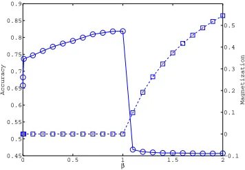
Figure 2: Temperature dependence of classification accuracy (circles) and magnetization (squares) for original method for 14 seed words.

ferromagnetic phase transition described above. The performance was assessed by using the General Inquirer labeled word list (Stone et al., 1966) as the gold standard. Of the 88,015 words in the network, 3596 were included in this list. Of these words, 1616 were positive, and 1980 were negative.

Testing was performed by varyingβfrom 0.1 to 2.0 by 0.1 and settingαto 1000. The num-ber of fixed seed words ranged from 2 to 14: {good, bad},{good, superior, bad, inferior}, and{good, nice, excellent, positive, fortunate, correct, superior, bad, nasty, poor, negative, unfortunate, wrong, inferior}.

0 0.5 1 1.5 2 0.45

0.5 0.55 0.6 0.65 0.7 0.75 0.8 0.85 0.9

Accuracy

β

−0.1 0 0.1 0.2 0.3 0.4 0.5

Magnetization

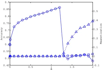
Figure 3: Classification accuracy and magnetization with improved method for 14 seed words. Circles ◦denote classification accuracy. Squaresƒand triangles △denote magnetization evaluated using all words and only the 3596 labeled words, respectively.

5 Improved Method

5.1 Attention to Largest Eigenvalue

The setting and results described above naturally led to the following considerations.

1. Because external fields are added to only a small number of seed words, a spin system operating at high temperature (smallβ) can be handled as a perturbed state from the trivial solution.

2. When the temperature is lowered from a sufficiently high value, classification accuracy monotonically improves until non-vanishing magnetization appears. This suggests that the ferromagnetic phase transition is the main cause of the drastic performance deterio-ration.

The second consideration suggests that the classification accuracy can be improved by pre-venting the ferromagnetic phase transition. Equations (7) and (9), in conjunction with the first consideration, imply that the phase transition is caused by divergence of the sensitivity matrix,(I−βJ)−1=PNµ=1(1−β λµ)−1xµ(xµ)tr, in the direction ofx1. This means that a

possible way to prevent this transition is to simply expurgate theλ1component from weight

matrixJ= (Ji j):

J′_=J−λ

1x1(x1)tr. (12)

Figure 3 shows the profiles of the classification accuracy and magnetization versusβfor the modified weight (Equation (12)) for 14 seed words. Similar profiles were obtained for the other two cases. Note that solving the mean field equation forJ′_{does not increase the} compu-tational cost significantly;x1can be obtained using the power method, for which the

compu-tational cost is similar to that of solving the original mean field equation. Theλ1x1(x1)trterm

Seeds SP LP Original Improved Improved (II)

2 70.0 74.8(0.6) 75.2(0.8) 84.5(1.2) 84.4(1.2)

4 70.0 74.2(0.7) 74.4(0.6) 83.5(1.2) 83.7(1.1)

14 74.2 81.6(0.9) 81.9(1.0) 86.2(1.2) 86.2(1.2)

Table 1: Optimal classification accuracy (%) for 2, 4, 14 seed words, and the cross-validation setting. “SP” corresponds to the method based on shortest path. “LP” corresponds to la-bel propagation. “Original” and “Improved” correspond to original method (Takamura et al., 2005) and one based on Equation (12). “Improved (II)” is same as “Improved” except that second largest eigenvalue component,λ2, is also removed from Equation (12). Values in

parentheses areβvalue at which accuracy was optimized.

As we speculated, the ferromagnetic phase transition was prevented, as shown by the mag-netization for “all words” (squares) in Figure 3. As a consequence, classification accuracy was improved beyondβ≃1.0. Classification performance was evaluated on General Inquirer as in the previous work (e.g., (Turney and Littman, 2003)). Table 1 shows the optimal clas-sification accuracy achieved for the original method (Original) and two improved methods, together with two existing state-of-the-art algorithms (SP and LP). SP is the method based on the shortest-path from seed words on the network (Velikovich et al., 2010). LP is the label propagation (Rao and Ravichandran, 2009). Note that, since we are interested in the impact made by the choice of algorithms, both of SP and LP were test on the lexical network that we used for our method, except that the edges with negative weights are removed because SP and LP cannot work properly with negative weights.3_{Also, although the label propagation by}

Rao and Ravichandran (2009) did not have the parameterβ, we introduced it to LP for the purpose of fair comparison. Its value is optimized on the test set.

The performance of Original was improved in all cases by using the proposed scheme (Im-proved). All the differences were statistically significant in the sign test with significance level of 1%. The result also shows that the improved methods are significantly better than the shortest-path based method and the label propagation.4 _{Note that the increase in}

ac-curacy compared with the values previously reported in some other papers (e.g., 82.8% (Turney and Littman, 2003) and 82.2% (Esuli and Sebastiani, 2005)) is substantial. The results with a few seed words (e.g., 2, 4, and 14) are more important since semi-supervised methods should be applied to resource-scarce languages or new domains where creating a large amount of seed words is not very practical. However, in order to examine the behavior of our method when we have many seed words, we employed 10-fold cross validation (i.e., approximately 3,200 seed words). The accuracy of 91.5% (Original) was slightly improved to 91.8 (Improved) and 91.9 (Improved (II)).

5.2 Removal of more eigenvalue components

Figure 3 also shows that the performance still deteriorated at a higherβvalue (1.3). To clarify the reason for this, we also plotted “selected magnetization” (triangles), which was evaluated

3_{The label propagation is not guaranteed to converge in the presence of negative weights.}

using only the 3596 labeled words for checking a possibility that a certain phase transition relevant to only the labeled words brings about the deterioration. The plot indicates that the selected magnetization bifurcates to a finite value forβ ≃1.3. This indicates that another phase transition occurred due to the second largest eigenvalue component,λ2.

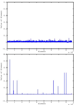
However, this indication is only partially correct. Figure 4 plots the profiles of the first and sec-ond eigenvectors. While the components of the first eigenvector (top) are evenly spread across almost all sites, those of the second one (bottom) are significantly localized at several sites. This “localization” feature is actually quite common for the eigenvectors of many other rela-tively large eigenvalues. Figure 5 plots the 30 largest eigenvalues and the inverse participation ratio (IPR), which is defined as

IPR= P

ivi4 (Pivi2)2

, (13)

for a real vector,v= (vi), of their eigenvectors (Biroli and Monasson, 1999). This quantity IPR

takes a value between 0 and 1. In particular, as the dimensionality tends to infinity, it remains positive for localized vectors but vanishes for spread ones, so this quantity is widely used as a standard measure for characterizing the localization property of high dimensional vectors. The plots in Figure 5 show that, althoughλ1is isolated, many other eigenvalues are distributed

in a rather degenerated manner and are accompanied by localized eigenvectors. The localized eigenvectors have non-negligible values only for a few elements. Therefore, removal of one of such components does not provide significant effects for most spins. This suggests that the bifurcation of the selected magnetization is caused by not only theλ2component but also

by many other components that are simultaneously excited atβ ≃1.3. Accordingly, little improvement in the classification accuracy can be gained by removing the components of the second largest eigenvalue component from the weight matrix, as shown in the rightmost column of Table 1. The performance was not improved significantly by further removing the third and the fourth eigenvalue components.

Note that most of the edges in the current network have positive weights, i.e., very biased to the same sign. This is the reason why the first eigenvector is not localized and the first eigenvalue is much larger than the others. Also, the localization of eigenvectors with large eigenvalues, which is observed except for the first eigenvalue in the current network, of-ten happens incomplex network. The theoretical background can be found in the paper by Kabashima and Takahashi (2012). Therefore, the characteristics of the network is not com-pletely accidental.

5.3 What is Essential?

0 1 2 3 4 5 6 7 8 9 x 104

−0.1 0 0.1 0.2 0.3 0.4 0.5 0.6

Element

Value of Element

0 1 2 3 4 5 6 7 8 9

x 104

−0.1 0 0.1 0.2 0.3 0.4 0.5 0.6 0.6

Element

Value of Element

Figure 4: Eigenvectors ofλ1(top) andλ2(bottom) of weight matrixJ.

Seeds 14 4 2

Accuracy 81.6(0.9) 74.2(0.7) 74.8(0.7)

Table 2: Optimal classification accuracy (%) of linearized model. Values in parentheses areβ at which accuracy was optimized.

high classification accuracy. For checking this possibility, we examined the performance of a simplified model defined by the linear approximation of Equation (9):

m= (I−βJ′₎−1_h0_{, (14)}

whereh0

= (h0i)is provided ash0i=αaiifiis included in the set of seed words and vanishes

otherwise. A power series expression,(I−βJ′₎−1₌P∞

n=0(βJ′)n, indicates that this can be

practically assessed by iterating the recursive equations:

mt+1_=mt_+ut _{and u}t+1_{= (βJ}′_)ut_{, (15)}

a sufficient number of times by setting the initial conditions asm0_=0andu0_=h0_{. This can}

0 5 10 15 20 25 30 0.7

0.8 0.9 1 1

Order of Eigenvalues

Eigenvalue

0 5 10 15 20 25 30

0 0.1 0.2 0.3

Order of Eigenvalues

IPR

Figure 5: 30 largest eigenvalues of J (top) and inverse participation ratio (IPR) for corre-sponding eigenvectors (bottom). Larger IPR suggests that the correcorre-sponding eigenvector is more localized.

one (Takamura et al., 2005). This suggests that much of the information needed to correctly classify words is included in the linear response of the spin averages to the polarities of the seed words at high temperature.

As shown in Figure 5, the eigenvectors of large eigenvalues, which are emphasized at low temperature, are mostly localized and could contain relevant classification information only for a few words that corresponds to non-negligible values of elements. Therefore, they are individually insufficient for correctly classifying most other words corresponding to negligi-ble elements. This means that, assigning polarities at high temperature so that information for all spin alignments is summed up with moderate probabilities is essential in the current spin-model-based method. This is achieved by assessing the linear response of the trivial so-lution to external fields representing the polarities of the seed words in the simplified scheme of Equation (14), and employment of the mean field equation (Equation (5)) offers a further gain under favor of the nonlinearity effect of tanh(·). This is in contrast to other approaches

0 1 2 3 4 5 6 7 8 9 x 104

−1 −0.8 −0.6 −0.4 −0.2 0 0.2 0.4 0.6 0.8 1

site

Spin Average

0 1 2 3 4 5 6 7 8 9

x 104

−1 −0.8 −0.6 −0.4 −0.2 0 0.2 0.4 0.6 0.8 1

Site

Spin Average

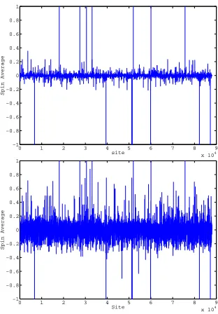
Figure 6: Spin averagesmiforβ=1.2 and 1.3 for 14 seed words. The mean of the absolute

value of|mi|increased more than ten times, from 0.0028 (β=1.2, top) to 0.0310 (β=1.3,

bottom).

is shown in Table 3. The comparison with the result in Table 2 suggests that the removal of the largest eigenvector also improves the linearized model. We note that the linearized model is almost equivalent to the label propagation (see the Taylor series in (Equation (6)); the dif-ference is simply the presence of the normalization step. In fact, the result of the linearized model (Table 2) is almost the same as that of the label propagation (Table 1). The experimen-tal result in Table 3 suggests that an idea similar to the removal of eigen components might also improve the label propagation, although we need to overcome the difficulty that the label propagation is not guaranteed to work properly if some edge weights are negative.

Conclusion

We have provided an analytical analysis of the behavior of a previously proposed spin-model-based method for constructing a polarity lexicon from the viewpoint of statistical mechanics.

Seeds 14 4 2

Accuracy 85.3(1.1) 83.8(1.1) 83.8(1.1)

On the basis of this analysis, we proposed a scheme for improving the performance of polarity lexicon extraction, i.e., removing the largest eigenvalue component from the weight matrix of the lexical network, the result is quite significant. For example, classification accuracy was increased from 75.2 to 84.5% for the case of two seed words without significantly increasing computational cost. This scheme also improves the linearized model.

We also examined the possibility of improving the performance further by removing more eigenvalue components. However, the resulting degeneracy of the eigenvalues in the weight matrix, which is accompanied by eigenvector localization, minimizes the gain improvement. In addition, we investigated a linearized model to characterize the classification performance and found that the linear response to the polarities of the seed words at high temperature contains essential information. While many methods have been proposed for binary classifi-cation, apparently most of them are based on optimization of a certain cost function or on achievement of the low-temperature state of the Boltzmann-Gibbs distribution. In general, high-temperature states are technically easier to handle than low-temperature ones because a greater variety of perturbative techniques can be used. The utility of the (linear) response in the high-temperature state shown here offers a novel promising approach to generic classifica-tion when labels are provided for a small fracclassifica-tion of representative instances.

The developed methodology can be employed for general purposes of assessing influences of a few representative nodes in a network via local communications. The Ising spin model or similar models including its linearized model are used in a number of tasks in natural language processing.

Future work includes more use of language data and development of applications using this polarity lexicon construction method as well as use of other approximation schemes such as ad-vanced Markov chain Monte Carlo methods in which equilibration is significantly accelerated by using extended ensembles (Iba, 1999).

Acklowdedgments

This work was partially supported by JSPS KAKENHI No. 22300003 and Mitsubishi Foundation (YK).

A Stability of Trivial Solution

Inserting Equation (4) into Equation (3) and setting hi to zero (i =1, 2, . . . ,N)yields an

expression of themean field free energy:

FMF(m) = −βX

i>j

Ji jmimj+

N X

i=1 X

Si=±1

(1+miSi)

2 log

(1+miSi)

2 . (16)

To examine the local stability of the paramagnetic solution,mi=0(i=1, 2, . . . ,N), we

evalu-ated the Hessian ofFMF(m):

H= ∂ 2_FMF(m)

∂mi∂mj

m=0

!

=−βJ+I. (17)

The solution is locally stable if and only if Hhas no negative eigenvalues. Equation (17) indicates that the eigenvalues ofHare given asβ−1−λµ(µ=1, 2, . . . ,N) using the eigenvalues

ofJ,λ1≥λ2≥. . .≥λN. Thus, asβincreases from a very low value, the stability condition

References

Alexandrescu, A. and Kirchhoff, K. (2009). Graph-based learning for statistical machine trans-lation. InProceedings of Human Language Technologies and the Annual Conference of the North

American Chapter of the Association for Computational Linguistics (HLT-NAACL2009, NAACL

’09, pages 119–127, Stroudsburg, PA, USA. Association for Computational Linguistics.

Biroli, G. and Monasson, R. (1999). A single defect approximation for localized states on random lattices.Journal of Physics A: Mathematical and General, 32(24): pages L255–L261.

Blum, A. and Chawla, S. (2001). Learning from labeled and unlabeled data using graph mincuts. In Brodley, C. and Danyluk, A., editors,Proceedings of 18th International Conference

on Machine Learning (ICML-2001), pages 19–26, Williams College, US. Morgan Kaufmann

Publishers, San Francisco, US.

Blum, A., Lafferty, J., Rwebangira, M. R., and Reddy, R. (2004). Semi-supervised learning using randomized mincuts. InProceedings of the 21st international conference on Machine

learning (ICML ’04), pages 97–104, New York, NY, USA. ACM.

Brody, S. and Diakopoulos, N. (2011). Cooooooooooooooollllllllllllll!!!!!!!!!!!!!! using word lengthening to detect sentiment in microblogs. InProceedings of the Conference on Empirical

Methods in Natural Language Processing (EMNLP’11), pages 562–570, Edinburgh, Scotland,

UK. Association for Computational Linguistics.

Choi, Y. and Cardie, C. (2009). Adapting a polarity lexicon using integer linear programming for dom ain-specific sentiment classification. InProceedings of the Conference on Empirical

Methods in Natural Language Processing, pages 590–598.

Esuli, A. and Sebastiani, F. (2005). Determining the semantic orientation of terms through gloss analysis. InProceedings of the 14th ACM International Conference on Information and

Knowledge Management (CIKM-05), pages 617–624.

Fellbaum, C. (1998). WordNet: An Electronic Lexical Database, Language, Speech, and

Com-munication Series. MIT Press.

Hatzivassiloglou, V. and McKeown, K. R. (1997). Predicting the semantic orientation of adjec-tives. InProceedings of the 35th Annual Meeting of the Association for Computational Linguistics

and the 8th Conference of the European Chapter of the Association for Computational Linguistics,

pages 174–181.

Hu, J., Wang, G., Lochovsky, F., tao Sun, J., and Chen, Z. (2009). Understanding user’s query intent with wikipedia. InProceedings of the 18th international conference on World wide web, WWW ’09, pages 471–480, New York, NY, USA. ACM.

Iba, Y. (1999). The Nishimori line and Bayesian statistics.Journal of Physics A: Mathematical

and General, 32(21): pages 3875–3888.

Kabashima, Y. and Takahashi, H. (2012). First eigenvalue/eigenvector in sparse random symmetric matrices: influences of degree fluctuation.Journal of Physics A: Mathematical and

Kaji, N. and Kitsuregawa, M. (2007). Building lexicon for sentiment analysis from massive collection of html documents. InProceedings of the Joint Conference on Empirical Methods in

Natural Language Processing and Computational Natural Language Learning (EMNLP-CoNLL),

pages 1075–1083.

Kamps, J., Marx, M., Mokken, R. J., and de Rijke, M. (2004). Using wordnet to measure semantic orientation of adjectives. InProceedings of the 4th International Conference on

Lan-guage Resources and Evaluation (LREC 2004), volume IV, pages 1115–1118.

Komachi, M., Kudo, T., Shimbo, M., and Matsumoto, Y. (2008). Graph-based analysis of semantic drift in espresso-like bootstrapping algorithms. InProceedings of the Conference on

Empirical Methods in Natural Language Processing, pages 1011–1020.

Li, X., Wang, Y.-Y., and Acero, A. (2008). Learning query intent from regularized click graphs.

InProceedings of the 31st annual international ACM SIGIR conference on Research and

develop-ment in information retrieval, SIGIR ’08, pages 339–346, New York, NY, USA. ACM.

Marcus, M. P., Santorini, B., and Marcinkiewicz, M. A. (1993). Building a large annotated corpus of english: The Penn Treebank.Computational Linguistics, 19(2):313–330.

Opper, M. and Saad, D. (2001). Advanced Mean Field Methods: Theory and Practice. MIT Press.

Rao, D. and Ravichandran, D. (2009). Semi-supervised polarity lexicon induction. In Pro-ceedings of the 12th Conference of the European Chapter of the Association for Computational

Linguistics (EACL’09), pages 685–682.

Schmid, H. (1994). Probabilistic part-of-speech tagging using decision trees. InProceedings

of International Conference on New Methods in Language Processing, pages 44–49.

Speriosu, M., Sudan, N., Upadhyay, S., and Baldridge, J. (2011). Twitter polarity classification with label propagation over lexical links and the follower graph. InProceedings of the EMNLP

2011 Workshop on Unsupervised Learning in NLP, pages 53–63.

Stone, P. J., Dunphy, D. C., Smith, M. S., and Ogilvie, D. M. (1966). The General Inquirer: A

Computer Approach to Content Analysis. The MIT Press.

Takamura, H., Inui, T., and Okumura, M. (2005). Extracting semantic orientations of words using spin model. InProceedings of the 43rd Annual Meeting of the Association for

Computa-tional Linguistics (ACL’05), pages 133–140.

Turney, P. D. and Littman, M. L. (2003). Measuring praise and criticism: Inference of semantic orientation from association.ACM Transactions on Information Systems, 21(4):315–346. Velikovich, L., Blair-Goldensohn, S., Hannan, K., and McDonald, R. (2010). The viability of web-derived polarity lexicons. InProceedings of Human Language Technology and the Annual Conference of the North American Chapter of the Association for Computational Linguistic

(HLT-NAACL 2010), pages 777–785.

Yu, M., Wang, S., Zhu, C., and Zhao, T. (2011). Semi-supervised learning for word sense disambiguation using parallel corpora. InProceedings of the 8th International Conference on