Implementing a lexicalised statistical parser

Implementing a lexicalised statistical parser

Corrin Lakeland, Alistair Knott Department of Computer Science

University of Otago New Zealand

{lakeland,alik}@cs.otago.ac.nz

Abstract

Statistical parsers are extremely complex sys-tems, yet papers describing them almost always only discuss theoretical issues instead of imple-mentation issues. This paper attempts to ad-dress the imbalance by describing the imple-mentation issues faced in building a state-of-the-art statistical parser. In the process, we will describe our own implementation of a statistical parser.

1 Introduction

Between 1996 and 1999, Michael Collins devel-oped a statistical parser (Collins, 1996; 1999) which has become tremendously influential in NLP. Collins’ thesis and published papers dis-cuss the theoretical underpinnings of his system in a great deal of detail; he devotes considerable space to describing and justifying the grammar formalism and the probability model which his parser uses. His description of his parsing algo-rithm is much less detailed; it is given as a set of pseudocode routines in an appendix. However, the scale and complexity of a lexicalised statis-tical parser is such that implementing this pseu-docode presents significant software engineering difficulties. The pseudocode actually disguises many of the interesting optimisations present in Collins’ system. As far as we can tell, no-body has published how to actually implement such a system. The aim of this paper is to de-scribe the important software engineering issues involved in implementing a lexicalised statisti-cal parser, using the parser we implemented as an example. What we found was that if you ever consider performance a secondary consid-eration then the parser will go so slow as to be impossible to debug. Because of this, we will concentrate on the efficiency of algorithms not so much to improve on Collins’, but just to get a working system.

We will begin in Section 2 by describing Collins’ probability model. In Section 3 we

de-scribe Collins’ parsing algorithm in high-level detail. The remainder of the paper describes our way of implementing the difficult parts of this algorithm. The chart data structure is de-scribed in Section 4; the generation of probabili-ties from the probability model in Section 5; the search strategy used by the parser is described in Section 6; Some general advice about soft-ware engineering in building a statistical parser is discussed in Section 7. And we conclude by noting that our parser performs almost the same as Collins’ in Section 8.

2 Collins’ probability model

The key idea in any statistical parser is to asso-ciate probabilities with grammatical rules. The probability of any given parse tree is then sim-ply the product of the probabilities of all the rules applied in creating this tree. However, in practice, the probability of a parse tree being the correct parse of a sentence depends not just on the rules which are applied, but on the words which appear at the leaves of the tree. To illus-trate, consider this well-known example of syn-tactic ambiguity:

(1) The man saw the dog with the telescope.

The PPwith the telescope can either modifythe

dog (as a relative clause) or the verbsaw(as an

adverbial). Intuitively, the latter reading should be preferred; we expect events of seeing to in-volve telescopes more frequently than dogs. The

notion of alexical headis useful in spelling out

this intuition. We expect a VP headed by the

verb saw to be quite frequently modified by a

PP involving the word telescope in a

represen-tative corpus, while we expect a NP headed by

dog only rarely to be modified by a PP

involv-ing the word telescope in such a corpus. We

2.1 Unary and dependency productions

How can we modify our grammar to include the appropriate lexical information? A useful

solu-tion, originally proposed by Blacket al.(1992),

basically involves a huge increase in the num-ber of phrases in the grammar. Instead of sim-ply having a phrase NP, we need one phrase for each possible headword of an NP: i.e. NP-headed-by-dog, NP-headed-by-telescope, and so on. At this point, unfortunately, we are faced with a data sparseness problem: we are unlikely to find sufficient counts for individual produc-tions, even with a very big corpus. The problem

is largely due toZipf ’s law; most words in the

language only occur very infrequently, so most grammatical categories, when tagged with an open-classed headword, will be fairly rare. The problem is compounded by the fact that many grammars allow a node to take several children. If each child is already rare, then the

combina-tion of nsuch children will be exponentially so.

With low counts, we cannot be confident in the probabilities we derive.

We will consider the problem due to Zipf’s law in Section 2.3. However, the problem of multiple children can be addressed by finding a way of splitting a parse tree into events that are smaller than single context-free rule appli-cations. A useful idea, originally proposed by Magerman (1995), is to break each single rule

application into several components: a unary

production which takes a phrase and

gener-ates its head constituent, and a set of

depen-dency productions which take a phrase and its head constituent, and generate the remain-ing child constituents, either to the left or the right of the head. The occurrence of a parent node decomposing into a set of children is now represented using the kinds of events shown in Figure 1.

Parent

Head

Parent

Left sibling . . . Head

Figure 1: Unary and dependency productions

The conditional probabilities we are inter-ested in are the probability of a head constituent given its parent (for a unary production) and the probability of a sibling constituent given its parent and its head (for a dependency pro-duction). These probabilities can be estimated from relative frequencies of events.

P(Head|P arent) = Count(Head, P arent)

Count(P arent)

The notation here needs some explanation. If you know the parent and you are trying to de-rive the probability for a given head, you can estimate the probability by counting the num-ber of times that head occurs as the head of that parent, and dividing by the total number of times that parent occurs. The categories ‘head’ and ‘parent’ are descriptions of constituents, which could be given at different levels of de-tail. If we are building a lexicalised grammar, these descriptions will each include a headword, as well as a grammatical category. The data sparseness problem due to Zipf’s law is now re-duced; unary productions only involve one lex-ical item, and dependency productions only in-volve two.

2.2 Collins’ probabilistic grammar

Collins’ probabilistic grammar is expressed in terms of unary and dependency productions, as just described. Of course, he includes more in-formation about these productions than we ex-pressed in the above equations. As well as a

head wordfor each constituent, he includes in-formation about the part of speech of this word: thehead tag. He calls the grammatical

cate-gory the head nonterminal, to distinguish it

from the tag. For the dependency productions,

he distinguishes betweencomplementand

ad-junct siblings of a head (a complement sibling

is tagged ‘-C’), and includes a

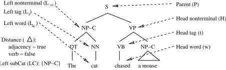
subcategorisa-tion framerepresenting the complements that the head needs. He also includes a measure of thedistancebetween the head and sibling con-stituents. To explain Collins’ representation of trees, we once again refer to a simple example tree — see Figure 2. In this figure, only the nodes pointed at by arrows take part in repre-senting events.

NP−C

DT NN VB NP−C

a mouse chased cat The

VP S Left tag (L )_t

Left nonterminal (L )NT Parent (P)

Head tag (t)

Head word (w) Head nonterminal (H)

Distance ( ): adjacency = true verb = false Left subCat (LC): {NP−C}

w Left word (L )

This figure shows the fields used to represent the dependency event of an NP-C attaching as a left sister to the head VP of a parent S node. Collins stores this event by encoding the terms pointed to with arrows in the figure. At this point, the event simply is the co-occurence of these values for these data fields. To represent a unary production, such as the generation of VP from the parent S node, we just need the terms on the right-hand side of Figure 2. To represent a subcat production, such as the generation of the VP’s left subcategorisation frame (in this case, a bag containing one item, NP-C), we use the same terms as the unary event, plus one additional field: a bag of nonterminals.

The probabilities we need to compute for unary, subcat and dependency productions can now be given more precisely, in the following three equations.

Punary(H|P, w, t)

Psubcat(LC|H, P, w, t)

Pdep(Lnt, Lw, Lt|P, H, w, t,∆, LC)

2.3 Collins’ event representation

To compute the above probabilities, we need to derive appropriate relative frequencies of events occurring in the WSJ corpus. Given that some events might be rare, or nonexistent, in this

cor-pus, Collins uses a backoff technique.

Basi-cally, we estimate the probability of a very cisely specified event by looking up a less pre-cisely specified one. For instance, the unary event in Figure 2 where it was decided VP should form the head of a sentence, would be as follows:

Punary(V P|S, chased, V B)

while a backed-off version of the event might

leave out the head wordchased:

Punary(V P|S, V B)

Collins makes use of three levels of backoff for all the events he represents: Level 1 contains all the terms pointed to in Figure 2, Level 2 drops a headword, and Level 3 drops everything ex-cept for nonterminals. To compute the proba-bility of an event, its numerator, denominator, and a weighting factor are looked up at all three levels of backoff, and the resulting probabilities are interpolated using the weighting factors. In summary, to derive the probability of an event, we must perform nine separate lookups of event counts in a database of events derived from the WSJ corpus.

2.4 Preprocessing the WSJ

The WSJ corpus is the main source of train-ing data for statistical parsers. The trees in the WSJ do not include information about head-words or complements, both of which are fun-damental to Collins’ approach. So Collins first has to add this information, using heuristics based on the syntactic and semantic annota-tions which are present. These heuristics are too numerous to doucment here, but a typical exam-ple would be that noun-phrases search right to left for their head child and prefer nouns. After applying the heuristics, he then has to trans-form the trees into a database of events to be counted when computing probabilities. While these preprocessing routines are relatively sim-ple compared to the parser, Collins has not released his preprocessor, and it is the least documented part of the system, so it is useful to document it; interested readers are referred to Lakeland (forthcoming), where preprocessing code is given in detail.

3 Collins’ parsing algorithm

We now present the high-level structure of the parsing algorithm.

Very briefly, in words, here is what happens.

In the top-level function parse, we begin by

initialising the chart with a set of complete

edges, each of which is one word from the input

string, and a set ofincomplete edges, each of

which is created by one or more unary produc-tions on one of the complete edges. A com-plete edge is one that will not be expanded

fur-ther. Then we call the function combine on

every set of adjacent edges in the chart. The

combine function attempts to join every pair of adjacent edges, using a dependency produc-tion, where the parent edge is incomplete and

the child edge is complete. This is done by

the functions join follow and join precede.

Whenever two edges are successfully joined, the new complex edge is added to the chart; then this edge is expanded using unary productions (considering both a single unary production and chains of two or three unary productions), and adds these to the chart. This is done by the

function add singles stops. The new edges

which have been added to the chart will be

found by subsequent calls tocombine.

parse(sentence)

initialise(sentence) for start = 0 to length

for end = start + 1 to length for split = start + 1 to end {

left = spanning(start,split) right = spanning(split+1,end) combine(left,right)

}

combine(left, right) { foreach (l left) foreach (r right) {

if (!l.complete && r.complete) joined = join_follow(l,r) if (l.complete && !r.complete)

joined = join_precede(l,r) add_singles_stops(joined) }

}

join_follow(left,right) { e = new edge(left)

e.add_child(right,at_end) e.prob *= right

e.prob *= dep_prob(left,right) chart.add(e)

}

join_precede(left,right) { (as per join follow) }

add_singles_stops(edges,depth=5) { if (depth == 0) return edges foreach (e edges)

e_stop += add_stop(e) foreach (e e_stop)

e_ns += add_singles(e)

add_singles_stops(e_ns,depth-1) }

add_singles(e) {

foreach (parent nonterminals) foreach (lc subcats)

foreach (rc subcats)

if(grammar(e,parent,lc,rc)) { result = unary(e,parent,lc,rc) chart.add(result)

results += result return results

}

Figure 3: Simplified parser pseudocode

Looking at the pseudocode it is hard to see where the implementation difficulty lies. The answer can be seen by counting loops:

parse contains three loops; combine contains two; add singles stops contains one; and

add singles contains three. Since these func-tions are all nested, the parser has nine nested loops. To address this complexity, two things are needed. Firstly, in general, we want to

im-plement everything efficiently, so that the

al-gorithm is as fast as possible. But as well

as efficiency considerations, we also need to build some genuine shortcuts into the

algo-rithm, by applying search heuristics which

discard edges unlikely to be in the final parse. Search heuristics are applied in two places in the

parsing algorithm: a beam search algorithm

is used in add singles stops to stop unlikely

unary productions from being generated; and

dynamic programming is used in the chart insertion routine to discard an edge if a more probable edge covering the same span already exists. These two issues — code efficiency and implementating heuristics — are what we focus on in the remainder of the paper.

4 The chart data structure

The goal of the chart is to store and provide access to all the edges covering each span of the input string. The grammar is very large because it contains a separate rule for each headword in each production, and because of this a great many edges cover each span. This means that the wrong choice of chart data structure will make parsing impossibly slow.

The most natural way of implementing such a data structure would be as a three dimensional array, in which the first two dimensions specify the start and end of the span respectively, and the last dimension stores the edges. Unfortu-nately, we do not know how many edges will be needed for any given span of the input string, which makes allocating such an array impossible (or at least extremely wasteful). To get around this problem, note that the flow of control of the parsing algorithm means that edges with a given start and end position in the input string are added consecutively. This means that we can store the chart as a huge one dimensional array

of edges, with a two dimensionalindex array

A related optimisation comes from noting

that the control structure of thecomplete

func-tion means that we always process one complete edge and one incomplete edge, so it would be more efficient if we could loop over all complete edges and all incomplete edges separately. It thus makes sense to have two separate charts, one for complete edges and one for incomplete edges.

Another optimisation relates to the use of a very simple dependency grammar within the

complete algorithm. Whenever two edges are joined, we must compute the dependency prob-ability for the join operation. If this probprob-ability is zero, there is no need to store the edge. In general we cannot predict when a dependency event will have a probability of zero in advance, but there is one exception: we can look at the nonterminal head of the parent and sibling, and if this combination was never seen in the train-ing corpus then we know the dependency event will have a probability of zero. The optimi-sation involves precomputing a simple depen-dency grammar specifying which nonterminal categories are found in dependency productions in the WSJ. (For instance, the top production in Figure 2 would allow a parent S whose head child is VP to have an NP-C as a left child.)

Now, in the combine function, we iterate over

every left and every right edge consistent with this simple grammar. To permit efficient access to grammatically consistent edges in the chart, we add a third dimension to the index array, to hold the edge’s parent nonterminal.

Another kind of optimisation in the chart comes from noting that it is possible for two different phrases to have the same representa-tion as events in Collins’ probability model. For instance, note in Figure 2 that Collins’ event

language makes no reference to the Det phrase

associated with the subject NP-Ccat. Since the

goal of the parser is to find the single best parse, if we ever have two phrases with the same rep-resentation at a given span in the chart, we can simply discard the one with lower probability; it will never be involved in the best parse of the

sentence. This is known as the Viterbi

opti-misation. A closely related optimisation is to discard any edge with a probability significantly lower than the best edge over this span, since it is very unlikely that a parse involving this edge will outscore a parse involving the most likely edge for this span. These last two optimisations

are examples of the dynamic programming

approach.

5 Computing probabilities

As mentioned in Section 2.3, to compute proba-bilities, Collins derives nine counts — that is, he looks up the number of times nine different sub-events have occurred in the database of sub-events derived from the WSJ corpus. This database cannot be stored as an indexed array since there is no obvious index; we therefore make use of the standard way of storing large data sets, hash ta-bles. The training data requires storing around fifty million events, and parsing a single sen-tence requires many millions of probabilities to be computed. Because performance is so critical it is worth being careful about the implementa-tion details.

Firstly, there is no need to store a hash table for every type of event. Instead we can use a sin-gle huge hashtable and include the type of event in the key. This does not make the system in-herently faster but does make it much easier to control the density of the hashtable which will lead to performance improvements. Secondly, it is conventional in hashtables to store both the key and value in the table so that hash collisions can be detected but here the hash key is many bytes and so it is more appropriate to just ig-nore collisions and accept that probabilities will be slightly incorrect. Finally, over ninety per-cent of probabilities computed in the parser are used more than once, so by storing all generated probabilities in a ‘cache’ hashtable, the speed of the whole system can be improved by an order of magnitude.

6 Implementing the beam search

The functionadd singles stopsincludes three

nested loops and is itself called recursively about five times. While none of these loops is dependent on the size of the input sentence

(i.e. the function is O(1)), an unconstrained

implementation would result in approximately

20005 _{edges being created (the number of}

non-terminals times the number of possible left sub-categorisation frames times the number of right subcategorisation frames, recursively called five times). Even if these edges were discarded by the chart on creation, the time taken to create them would make it impossible to parse a sim-ple sentence. To resolve this, Collins only ex-pands edges likely to be part of the final parse. Collins’ thesis notes he uses a constrained best

process. The benefit of this is that instead of an unmanageable number of nodes being cre-ated, perhaps only a few hundred are created (of which dynamic programming in the chart will still discard all but a handful).

Search generally involves creating new nodes for each child being expanded. But as is men-tioned in Section 7, allocating memory is a com-putationally expensive operation and is unde-sirable in a program where efficiency is

criti-cal. Since a beam always has exactly n nodes

on it, it seems intuitively obvious that beam-search could be implemented without allocat-ing memory but it proves surprisallocat-ingly difficult to do efficiently. Our implementation of beam

search uses skiplists (Pugh, 1989). Skiplists

are a variant on linked lists in which a number of ‘next’ pointers are kept on each node instead of just one. These extra pointers allow the al-gorithm to ‘skip’ along the list and lead to

in-sertion and access times of O(lgn) (the same

as binary search, but much simpler to imple-ment). As an extension to Pugh’s idea, we im-plemented double-ended skiplists (analogous to

doubly-linked lists). This givesO(1) access and

insertion to both the start and end of the list. Having developed a suitable data structure,

we apply it to beam search. By allocatingn+ 1

nodes for a beam of length n, we can

pro-videadd singles with an empty node in O(1) by simply returning the last node in the list

(technically, these functions are not O(1) but

O(lg(lg(n)) due to pointer management code,

but this closely approximates 1 for even huge values of n). In practice, insertions are almost always at the start or the end of the list (both

approximately O(1)). When they are at other

parts of the list, insertion is an O(lgn)

opera-tion.

The obvious comparison for this approach would be using a heap, as a heap is the data structure most commonly used to implement

priority queues. Using an array based heap

(since the size of the queue is bounded) we can

access the front inO(1), but to remove the last

node and reinsert is O(lgn). Compared to this

implementation, skiplists are somewhat more

efficient atO(lg(lgn)).

Overall, double-ended skiplists have proven to be an interesting and efficient method of

im-plementing beam-search for largen. Wherenis

low, it is probably more efficient to simply use a doubly-linked list but Collins’ noted he used a beam size of 10,000, and so a more sophisticated

approach is called for. After implementing the skiplists search, Collins released his code and it is very interesting to compare his approach; it turns out he does not actually implement clas-sical beam-search, but instead uses an array of edges being expanded with a threshold — if an edge is a certain amount worse than the best then it is discarded. This is significantly simpler and somewhat more efficient than my approach. However it would perform very poorly anywhere where the heuristic evaluation improves as we move away from the start state.

7 General software engineering issues

The core difficulty in implementing a statistical parser is that it processes a vast amount of data. The event file created by the preprocessor con-tains perhaps fifty million events; the beam is searching through perhaps ten thousand local possibilities; and the chart contains hundreds of thousands of ambiguous partial parses. All this means that we must keep code as efficient as possible throughout the development pro-cess, or the parser will simply fail. In addition, that sophisticated code and data file verification techniques are crucial, because small bugs can have far-reaching consequences. In this section, we present some of the software development lessons we have learned in building our parser.

7.1 Start by solving a smaller problem

A lexicalised statistical parser is a very com-plex system, where a single poor choice results in a program that is too slow to test. How-ever, building a part-of-speech (POS) tagger has many of the same issues as a statistical parser

but without the asymptotic complexity. We

found it was useful to begin by building a full reimplementation of Collins’ probability model which was only used for POS tagging (Lakeland and Knott, 2001). This enabled about half of the system to be verified.

7.2 Choice of programming language

Initially our parser was implemented in LISP, because it is a language ideally suited to both

tree processing and prototyping. It was far

can be hacked into the control structure of the program.

It is worth explaining why direct memory management is essential. Allocation of memory is an extremely slow function and any program desiring efficiency must not allocate memory in-side its inner loop. By preallocating data struc-tures (e.g. allocating all the memory for the chart and the beam before parsing begins), it is possible to avoid any memory allocation during the core parsing loops, saving a great deal of

time. Languages such as Java, C# _{and Python}

are therefore a bad idea; their automatic mem-ory management (normally a key selling point) is precisely what we need to sidestep to im-plement an efficient parser. Consequently, like Collins, we chose to implement the parser in C, which provides low-level memory management support. (However, for preprocessing the cor-pus, we stuck with LISP, since it is not time critical.)

7.3 Version control

Anybody building a nontrivial program will use a source code control system such as CVS or subversion. But we found that naive use is in-sufficient – for instance we frequently found im-provements to the preprocessor would break the parser since it depended on the older format for the data files. We also needed to make use of ‘branching’.

Another related step was the development of a build script. There are a large number of steps involved in converting the treebank and other data into a format suitable for parsing. It is rel-atively easy to perform these steps sequentially. However that means any change to one of the earlier steps (such as a tweak to the tokeniser) requires every subsequent step to be repeated. Since there is usually output from the previous version lying around, it was often the case that output files from different versions of the code would be used at the same time — leading to subtle errors.

Finally, version control only applies to files but we often found that we needed to write

almost identical blocks of code, but often we could not write the code as a general func-tion which decided its behaviour based on ar-guments and writing the same code twice in-variably leads to bugs being fixed in one version but not in another. Our solution to this was to use source code preprocessing so that our sin-gle ‘meta’ version generates multiple functions,

each with slightly different logic. We used the toolfunnelwebfor this purpose.

7.4 Efficiency versus debuggability

It is often the case that the most efficient data structure is harder to debug. For instance, our hash keys can be easily compared to the data used in generating the key and so a bug in key generation is easily identifiable while Collins’ keys bear too little correspondence to data and so cannot be easily debugged but they can be generated faster. Similarly, Collins uses array offsets to refer to edges where we use pointers which will make our code slightly faster, but it makes tracking an edge through parsing much easier in Collins’ system.

‘Magic numbers’ are another area in which bugs can easily creep into the system — for in-stance, setting the maximum number of nonter-minals to 100 might be correct at first, but later adding -C complements could easily overflow this and lead to data corruption. We managed to avoid many of the problems here by automat-ically generating the declarations of constants from the input files, so any change to the in-put files will automatically appear in the source code. Similarly, many functions in the probabil-ity model take a dozen or so parameters and get-ting these in the wrong order will not cause any typecast errors since they are all integers, it will just generate invalid output. This problem was avoided by implementing basic datatypes as dif-ferent classes so that incorrect orders does result in typecast errors. Curiously, Collins uses magic numbers everywhere and I often wondered how he managed to debug them in his parser.

7.5 Debugging methodology and test suites

In order to facilitate this, after testing ev-ery function we wrote an automated test suite that rechecks functions every time the system is built. For example, the probability model can be checked by comparing the counts it

de-rives to those produced with grep. If a bug

is later introduced in the input to this func-tion then it will likely cause some testcase to fail. Similarly, the system is liberally scattered with assert statements that perform every-thing from internal bounds checking to checking

that the skiplist is in sorted order and still hasn

elements. As a last resort, we also made

exten-sive use of the memprotect kernel call to lock

any data that was not currently being edited (such as the hash tables). This allowed us to catch a number of bugs where we had forgotten an assertion.

A final comment is that we found high-level debugging to be much less useful than low-level debugging. For instance, by examining the sen-tences the parser performs poorly on it may be possible to infer it has a problem. But this ap-proach turned out to be significantly more time-consuming than simply verifying every function independently, mainly because the parser was too big to find where the bug was after the high-level approach found the existence of a bug.

8 Conclusion: results of our own parser

The parser we implemented performed almost identically to Collins’ as regards precision and

recall (84.5% as opposed to 85%). In over

95% of cases, our parser produces exactly the same output as Collins’, with differences partly caused by small undocumented tweaks Collins made, such as using the headword from a child instead of the parent during coordination, and partly due to some late design changes made as our understanding of Collins’ algorithm im-proved. Our system is significantly more mod-ifiable than Collins. This is because it was de-signed with that in mind, and also because all of the seperate components used are tightly seper-ated out into different classes with well specified interactions. Because of this, my system is well suited as a platform for further research.

References

Black, E., Jelinek, F., Lafferty, J., Magerman, D., Mercer, R., and Roukos, S. (1992). To-wards history-based grammars: using richer models for probabilistic parsing. In M.

Mar-cus, editor, Fifth DARPA Workshop on

Speech and Natural Language, Arden Confer-ence Center, Harriman, New York.

Collins, M. (1996). A new statistical parser

based on bigram lexical dependencies.

Collins, M. (1999). Head-driven statistical

mod-els for natural language parsing. Ph.D. thesis, Computer Science Department, University of Pennsylvania.

Lakeland, C. (forthcoming).Lexical Approaches

to Backoff in Statistical Parsing. Ph.D. the-sis, Department of Computer Science, Uni-versity of Otago.

Lakeland, C. and Knott, A. (2001). Pos

tagging in statistical parsing. In Proc. of

the Australasian Language Technology

Work-shop, Sydney, Australia.

Magerman, D. M. (1995). Statistical

decision-tree models for parsing. In Proc. of the 33rd

Annual Meeting of the Association for Com-putational Linguistics. Cambridge, MA, 26– 30 Jun 1995.

Pugh (1989). Skip lists: A probabilistic

alterna-tive to balanced trees. In WADS: 1st