F20 8077 An Introduction to Engineering Analysis for Computers 1961 pdf

General Information Manual

An Introduction to

General Information Manual

An Introduction to

CONTENTS

SECTION I: INTRODUCTION .

Historical Notes. . . . The Digital Computer. . . .

Storage . . . . The Stored Program Addresses

Control Unit Arithmetic Unit Binary Arithmetic Input and Output Summary. Exercises . . . .

SECTION II: THE FORTRAN LANGUAGE Exercises

SECTION III: SOME NEW AND OLD CONC EPTS Block Diagramming

Subscripting . . . . Absolute Value . . . . Floating Point Arithmetic Errors

Recursion Formulas . .

Algorithms . . .

Complex Number Calculations Transformations and Identities . Exercises

SECTION IV: PRINCIPLES OF ITERATION Arithmetic, Mathematics and the Computer

Numerical Analysis . . • .

Algebraic Equation

Equations of Calculus. . . Iteration Type Problems Exercises . . . .

SECTION V: MATHEMATICAL MODELS Solenoid Design . . . .

Heat Transfer Problem . • Rocker Arm Cam Problem

S pring Problem . . . • . . Pitman Arm Stress Analysis .

Automobile Suspension . ~

Spring Stress Analysis Problem Vehicle Simulation Model . . . . . Exercises

SECTION VI: SELECTED MATHEMATICAL TOPICS Matrix Inversion . . . •

Eigenvalue Problem . . • • . Partial Differential Equations

1 1 6 6 7 8 8 9 · 10 11 · . 11 12

· . 14 21

· . 22 · • 22 • • 25 · 26 26 · . 27 · • 27 • • • • 28

• • 30 · . 31

32

. . • • • 34

• • 34 • • 37

• • 37 · • 39 · • 39 · 51

· • • • 53 • . • 53 . • • • • 54 • • 58 61 · 67 69 · . . 71 • • 73

77

Potential Problem

Temperature Distribution Problem Exercises. . . • . . • . • .

SECTION VII: EMPIRICAL RELATIONSHIPS Functions of a Single Variable

Table Lookup . . . . • .

Data Fitting . . . . Functions of Multiple Variables

Table Lookup . • • .

Data Fitting Dimensional Analysis Probabilities . Exercises.

SECTION VIII: OPERATIONS RESEARCH Job Shop Simulation . • . . . • . . Inventory Control . .

Linear Programming . . • • . • .

Exercise

APPENDIX I: ANSWERS TO SELECTED EXERCISES

APPENDIX II: BIBLIOGRAPHY

85

• 88 · 91

· • 93 · • 94 · 94 • • 95 97 • . • 97 • . 98 . . . 100 · .103 · .105

· .107 · .110 · .113 · .120 · .124

· .126

SECTION I: INTRODUCTION

Historical Notes

To most engineers practicing in industry the high speed digital computer is an unknown quantity. Just five years ago an engineer's chances of having an introduction to computing while in college were slim indeed.

Today virtually all the major engineering schools in this country have access to digital computers. Within the next five years the engineer who graduates without an introductive course in the use of computers will be the exception.

The growth in the use of the digital computer has been tremendous. The first large scale digital computers appeared in the early 1950s as an out-growth of interest generated through the use of punched card calculators such as the IBM Card Programmed Calculator. Over 4,000 digital com-puters were installed in 1960, varying from small engineering machines to very large commercial and scientific data processing systems.

Like all technological developments, the digital computer has its historical antecedents. Computing itself is one of the oldest human activities, re-quired by all civilizations for the conduct of business and the development of sciences. One of the most practical inventors of recent times, Charles Kettering, inventor of the auto self-starter, made the statement, "You cannot understand a thing unless you can give it a number." In many ways civilization has always been tied to this need for quantitative or numerical description.

In fact, the oldest surviving written document is a set of business records kept by a Sumerian of Mesopotamia 5, 000 years ago.

The development of computing methods was painfully slow. Perhaps this was due in part to the unfortunate choice of number symbols (e. g., Roman numerals) and of number bases (e. g., the Babylonian choice of the base 60). Gradually the Arabic numeral system and the base 10 won out as modes of computation, although vestiges of other systems remain impor-tant (e. g., Roman numerals for date inscription, and base 12 for the inches in a foot measure).

Perhaps, too, this slow march forward in computing methods was due to the fact that they were not greatly needed, for certainly the first big breakthrough occurred when the science of astronomy depended on tremen-dous computing efforts for its advance. In the 16th century these efforts were greatly eased by the development of logarithms by Napier and Briggs. Considering the size of numbers used in astronomy, one can easily see why the logarithmic transformation which allows multiplication and division to be handled as addition or subtraction was a significant contribution.

A most interesting personality in the science of machine computation was the misunderstood genius Charles Babbage of England, whose major work was done in the middle 1800s. During his lifetime, Babbage conceived and designed on paper what he termed the analytical machine. In virtually all respects this machine was to perform like the modern digital computer, except that it was to be mechanical rather than electronic. The fasci-nation which Babbage r s work holds for present-day computer people can

be explained when some of his ideas are discussed.

For example, his analytical machine was to have the ability to "remember" 1, 000 numbers up to 50 digits in length. This capacity is greater than that of many electronic computers now in existence. His machine was to be controlled by punched cards, an idea which he borrowed from the use of cards in controlling looms. In the light of the present day role of the punched card in data processing, Charles Babbage seems a prophet.

It is a certainty that if Babbage had been content to build on a smaller scale rather than design on such a grandiose level, the science of com-puting would have profited greatly in the 100 years between his analytical machine and the present day. As it was, however, Babbage never com-pleted his machine, and in general we are aware of his genius primarily through the writings of an admirer, one Lady Lovelace, who wrote most descriptively of the design and philosophy of the analytical machine.

In truth one of her statements might stand as a preface to the study of the modern electronic computer: "The Analytical Engine has no pretensions whatever to originate anything; it can do whatever we know how to order

it to perform. "

Charles Babbage did successfully build what is termed a difference machine for the computation of tables. Many of the early efforts in machine com-putation took this line of construction of machines to do particular comput-ing jobs. A simple example will illustrate a principle made use of in such machines:

To construct a table of values for

Differences

M F 1st 2nd 3rd

0 0

2

1 2 8

10 6

2 12 14

24 6

3 36 20

44 6

4 80 26

70 6

5 150 32

102

6 252

The third difference is a constant. The table can be completed by working back from the third difference to compute further entries of F by simple additions. It is relatively simple to build a machine to perform these simple additions to successive columns.

The principle used here has been to take successive derivatives of the function F.

The third derivative is the constant 6.

A great many of the functions for which tables are desired in the fields of navigation, astronomy and surveying can be handled by such techniques. The literature of computing abounds with the application of difference procedures.

However, modern computers are a far cry from the difference machines of Babbage I s day.

At about the same time Babbage was laboring with his "Analytical Engine, " George Boole, an English mathematician, was laying the foundation for later developments with his study of the algebra of logic. Boolean algebra is the foundation of work in machine logic (so necessary in the design of digital computers) and has contributed in the logic of business contracts and law (equally necessary in many areas of data processing).

In the 1930s the work of modern mathematicians, in particular the late John von Neumann, spurred interest in the possibilities of machine com-putation. Various computers - both special-purpose analog devices and

at universities. Harvard and MIT were the centers of most of this activity. World War II was a catalyst to machine computing in that the military technological advancements demanded tremendous computational facilities. By the end of the war the logic for construction of a general-purpose digital computer was fairly well specified.

As makers of computing devices for accounting and business, manufac-turers of business machines became involved in this effort of machine computation. The first large scale general-purpose digital computer was built by IBM for use in scientific research. Known as the IBM Automatic Sequence Controlled Calculator, it was presented to Harvard in August 1944. Its capacities were not surpassed until the IBM Selective Sequence Electronic Calculator was dedicated in January 1948.

The SSEC was dismantled to make room for its successor, the IBM 701, announced in March 1953. At this time the general belief was that a few large scale machines could handle all the computing needs of the country. The demand for more and more machines when the first few became available soon made apparent the vast needs for computation in both tech-nology and business. Today these needs have been multiplied by further recognition of existing needs and the discovery of new approaches to old problems.

How does this affect the engineer?

The field of engineering analysis for computers has experienced tremen-dous growth in the past five years. The advent of the electronic computer has created a new approach to engineering problems. The costly "build and try" method is now often replaced by "construct mathematical model and simulate."

In some respects this represents a return to the textbook for the engineer. He must describe the physical problem by means of a mathematical model. Then the computer can operate the model and describe operating results. The real power of the computer is that it will quickly describe operating results for many sets of operating conditions.

Many articles have been printed in professional publications on the solu-tion of difficult engineering problems by the use of electronic computers. These applications have only scratched the surface of possible engineering use, and a lack of knowledge and experience prevents the full use of the computer as an engineering tool. The engineer is simply not aware of what a computer can do for him. It is highly desirable, therefore, that every engineer understand how problems can be described for handling by electronic computers.

It is convenient to think of computer problems as falling into one of two classes:

1. Obvious computations

2. Iterative problems

Obvious computations are those which have in the past been handled by slide rule or paper and pencil. They also include those for which the tech-nique of solution, while known, has required too much computation to tackle.

Iterative problems comprise a large area, mostly unexplored. To explain this, the question should be asked, "What is the function of the engineer today?"

The engineer is a person who builds physical systems to do particular jobs. If a particular construction does not work, modifications are made until it does work. These modifications are often the result of vague ideas. Engineering is largely by trial and error.

A very obvious conclusion which one reaches in talking with engineers is that they employ a minimum of their textbook analysis techniques. Math-ematical approaches soon pick up dust on the engineer's worktable. Why? One reason· is that real life simply does not fit the pat equations of the textbooks. Often the basic difference is that in a textbook it always seems possible to apply mathematical techniques and arrive at solutions of the kind

x = f (y, z)

where the value of the variable of interest can be determined simply by plugging in known values for y and z on the right-hand side. However, in real-life engineering, often the problem becomes stated as

x = f (x, y, z)

where x is on both sides of the equation. x cannot be solved for explicitly; that is, there is not enough information to remove x from the right-hand side. The problem is too complex.

This problem can usually be handled mathematically by estimating the value of x, testing the estimate, and, if it is wrong, making a better estimate. Essentially, numerical analysis (in computer mathematics) is the science of making progressively better estimates. To estimate

repeatedly is to "iterate." This iterative idea is the heart of the computer approach, whether for the simplest cam problem requiring algebra, or for the most complex nuclear problem involving sets of differential equa-tions.

The Digital Computer

The layman I s image of the electronic computer contains a pinch of mystery, a dash of magic and a number of false analogies to human beings. These misconceptions have in some cases been nurtured by computer manufac-turers through their use of such terminology as

1. Memory - for that part of the computer which stores information.

2. Nerve Center - for that part of the computer which controls its operation.

3. Brain - for that part of the computer which accomplishes arithmetic and logical operations.

While these analogies do help in understanding the functions of some of the components of a computer, they also tend to develop a camouflage of complexity .

The computer, like the automobile, airplane, nuclear reactor or any other engineering achievement, is the product of a group of engineers. (It should not be surprising that in developing this product, engineers have used other computers to solve some of their design problems.) As in the case of the automobile and airplane, a person need not be capable of designing and building a computer in order to use one. Few persons who drive an auto-mobile are capable of describing the complex of gears, rods and shafts that allow a rotation of the steering wheel to change the direction of travel. This, however, does not prevent them from becoming excellent drivers. Similarly, a general knowledge of the functional components of a computer is all that is needed to use one effectively. Once the basic concepts are understood, greater familiarity is easily developed through experience.

What are these basic concepts? To answer this, consider the basic com-ponents of a computer.

STORAGE

That part of a computer which most differentiates it from a calculator (desk-type, slide rule, adding machine) is its storage - or, to use the unapproved analogy, its "memory."

digits and call them out of storage whenever they are needed in a calcula-tion.

THE STORED PROGRAM

The ability to store large amounts of data that is to be used in or has been developed by calculations is only part of the function of storage. Equally significant is the fact that the computer also contains within storage the program for the calculations to be performed.

Data

STORAGE

Program

A program is made up of instructions which, when acted upon by the com-puter, cause it to go through the sequence of operations necessary to arrive at a meaningful result. A single instruction may:

1. Cause data to be brought into storage from some external source, such as a card reader.

2. Cause a specified arithmetic operation to be performed on selected numbers.

3. Constitute a logical test to determine what part of the program should be performed next.

4. Cause results to be sent from storage to a recording device, such as a typewriter.

After both the data to be operated upon and the program which describes the operations are in storage, the computer is free to proceed with a series of calculations at its own natural speed. For present-day machines, this may be from 50 to 500, 000 additions per second.

This leads to another salient fact: A computer can change or modify its own program! Since the program is stored in much the same form as data, one portion of a program may be a sequence of operations which will examine another portion of the same program and change it by arith-metic or logical manipulations. What advantage is to be gained from this?

First, it means that one set of instructions can be used to operate on a number of sets of data stored in different locations in storage. As each set of data is processed, the program is changed to refer to the next set of data.

y = x2 , for x ~ 1

y = -x2+4x-2, for x > 1.

At the point in the calculations where the value of x becomes greater than 1, that portion of the program involved in the evaluation of y can be changed to use the second of the two equations. This change might be accomplished by replacing one set of instructions with a new set stored elsewhere for that purpose, or it could also be done by causing the computer to select one of two instruction sequences on the basis of whether x is greater than 1 or not greater than 1.

ADDRESSES

To be able to select the item of data or the instruction to be operated upon next, the computer must be provided with a means of locating the desired information in storage. For this reason, storage is divided into units and each unit is identified by an address. Different computers are designed with different-size units of storage. The basic unit may vary from one decimal digit (as in the IBM 1620) to 36 binary digits (as in the IBM 7090). In other computers, units of one alphameric character (that is, a decimal digit, letter of the alphabet, or special character) or ten decimal digits are used.

Whatever the size of the basic unit, each is assigned a numerical address which identifies the location. Manipulation of the data stored in a location is accomplished through the use of the address corresponding to the loca-tion.

CONTROL UNIT

The control unit of a computer provides the means whereby the stored program causes the desired operations to be performed in the sequence specified. The control unit reads an instruction from storage, examines it, sets up the circuit conditions to perform the operation, and, when the operation is completed, reads the next instruction from storage and re-peats these steps.

CONTROL

i

STORAGE

ARITHMETIC UNIT

This component contains the circuitry which performs arithmetic on num-bers taken from storage. It usually includes a limited amount of storage in which to hold the operands involved in the arithmetic.

CONTROL

STORAGE

ARITH1v1ETIC

At this point it is wise to pin down the kind of arithmetic accomplished in a computer. The two basic types of computers - analog and digital -have different ways of accomplishing arithmetic. The analog computer performs arithmetic by measuring, the digital computer by applying a set of rules to the numbers involved.

To illustrate, suppose that two numbers to be added are 56.8 and 29.5. A simple analog device for obtaining the sum would be a ruler divided into 100 units. The ruler is laid on a piece of paper and marks are made on the paper next to the 0 and 56.8 points on the rule. Then the ruler is picked up and the zero point of the ruler is placed next to the mark on the paper representing the 56.8 point. Now a third mark is made on the paper opposite the 29.5 point on the rule. All three marks, of course, are made to fall on a straight line. Finally, the distance between the first mark and the third is measured with the rule. Because of the possibility of measure-ment errors inherent in such a procedure, the result obtained might per-haps be 86.2.

o 56.8

X

x

I

I

0 29.5

x

A schoolboy. will add the numbers by writing one under the other and ap-plying a set of rules involving such things as the sum of two digits and how to handle the carry when the sum is greater than 9. Thus,

1 1 5 6.8 2 9.5 8 6.3

This is the technique used by the digital computer - that is, the digital computer performs arithmetic by the application of a set of rules. There is no error inherent in such a technique.

BINARY ARITHMETIC

While on the subject of arithmetic, it is well to dispense with another question which is bound to arise in the reader's mind: What is binary arithmetic?

A problem in computer design that the engineer may have recognized by now is that to store and manipulate decimal digits requires some device capable of assuming ten stable and unique states - one state to represent each of the digits 0 to 9. While such devices are available (the notched wheels in a desk calculator are an example)p they lack the speed of opera-tion and small size necessary for a computer. Furthermore, they don't fit into an electronic system.

Many electronic devices are available, however, which can assume two stable and unique states. A tube, for example, can be conducting or non-conducting; a magnetic field can have clockwise or counterclockwise rotation; a pulse can be transmitted or its transmission can be blocked.

The computer designer has at his disposal, therefore, a number of devices and techniques for operating in a number system with the base 2 - the binary number system. The rules for arithmetic are also much simpler in the binary number' system than in the decimal system (base 10) which we are accustomed to using.

ADDITION TABLES

o

o

o

1 10

MULTIPLICATION TABLES

o

o

o

o

1

o

DECIMAL BINARY DECIMAL BINARY

o

1 1 6 110

2 10 7 111

3 11 8 1000

4 100 9 1001

As far as the user is concerned, it is not necessary to be familiar with the binary nature of the computer. The computer is capable of translating the engineer's language to its own before starting a program and performs the reverse operation when communicating its results to the engineer.

INPUT AND OUTPUT

So far, the methods for getting data and programs into the computer and for getting the results out have been ignored. Every computer must have a means for communicating with the outside world.

Typical input devices are punched card readers, paper tape readers and manual keyboards. Card and paper tape punches, typewriters and printers are typical output devices. Magnetic tapes and magnetic disks provide a means of storing data

CONTROL

INPUT STORAGE OUTPUT

ARITHMETIC

externally from the computer in a form which allows rapid re-entry.

The use of input-output devices is under control of the stored program. For example, an instruction to read a card will cause the card reader to start up, feed and read one card and transmit what has been read into storage.

SUMMARY

Thus there are five basic components of a computer:

Exercises

2. A means of controlling the overall action of the system.

3. Devices for performing arithmetic and other operations required in manipulating the data to obtain desired results.

4. A way of getting information into the computer.

5. A way of getting results out of the cumputer.

1. The decimal system has as its base the number

---2. The numeral system commonly used is the

-numeral system.

3. Logarithms aid greatly in doing the arithmetic operations of

and when working with many significant

: :

-figures.

4. Difference principles were used in the construction of

---5. The first large scale computers were electromechanical in design;

the middle 1950s saw the common use of the design,

and the computers being designed and built now have solid-state (e. g., tranSistorized) components.

6. The general iterative problems may be stated by a formula of the type

-7. Three computing devices with which most engineers are familiar

are , and

---8. One of the difficulties in predicting the behavior of complex systems is that engineers have trouble maintaining the

---9. Two economic aspects of a problem which most engineers are

concerned with are • and

10. Two types of information stored in the memory of a computer

are and

---11. Modification of the by another set of operations

is important for repetitive and logical abilities of a computer.

12. The unit interrogates the memory for

information as to what to do next.

13. The gives the physical location of

infor-

~~---mation in memory.

14. An analog device computes by , a digital

15. The binary system is a number system of base

- - - ,

16. Because the information in memory may be changed at any time, the digital computer is called a

---17. The physical property of is what makes a

SECTION II: THE FORTRAN LANGUAGE

FOR TRAN (FORmula TRANslation) is a language which allows the engineer to communicate a problem to a computer for solution.

FOR TRAN is not the natural language of a computer, nor is it the natural

language of the engineer. Rather, it is a compromise between the two.

To satisfy the computer, it uses symbols that the computer can understand and requires that the rules for their use be closely followed. To satisfy the engineer, it eliminates as many of the detailed computer control opera-tions as possible from the job of writing programs and uses a problem statement format close to that of the mathematical equation.

The engineer describes his problem in the FORTRAN language; what he writes is translated into the natural machine language of the computer to be used in obtaining the solution. The translation is accomplished by the computer itself with the aid of a program called the FORTRAN Processor. The resulting machine-language program is then ready to be used to obtain the solution. This diagram illustrates the procedure:

0

..

....

Problem r '

...

•.. in FORTRAN FORTRAN

language Processor

"

(

machine-language program

~,

Input

.

...

..

...

data

~

Sfatements are the sentences of the FORTRAN language. They may:

1. Define the arithmetic steps which are to be accomplished by the computer.

2. Provide information for control of the computer during the execution of the program.

4. Specify certain additional facts such as the dimensions of a variable which appears in the program with subscripts.

Because the printer and typewriter on a computer print only in upper-case letters, have a limited number of different characters, and are incapable of properly showing exponents and subscripts, FORTRAN statements at first appear somewhat confusing.

An example of an arithmetic statement as it would appear on a FORTRAN coding sheet is:

ROOT:::: ( -B+SQRTF(B**2-4. *A*C»/(2. *A)

Translated, this says:

The quantity to be known as root is equal to - that is,

can be determined by - evaluating

where A, B, C are given values stored within the computer.

Arithmetic statements look like simple statements of equality. The right side of all arithmetic statements is an expression which may involve parentheses, operation symbols, constants, variables, and functions, combined in accordance with a set of rules much like that of ordinary algebra. The symbols + and - are employed in the usual way for addition and subtraction. The symbol * is used for multiplication, and the symbol / is used for division. The fifth basic operation, exponentiation, is rep-resented by the symbol **. A **B is used to represent A to the exponent B (that is, AB).

The FORTRAN arithmetic expression

A **B*C + D**E/F - G

will be interpreted to mean

That is, if parentheses are not used to specify the order of operations, the order is assumed to be:

1. exponentiation

2. multiplication and division

3. addition and subtraction

(A(B + C»D is written in FORTRAN as

(A*(B + C» **D

There are just three exceptions to the ordinary rules of mathematical notation. These are:

1. In ordinary notation AB means AeB or A times B. However, AB never means A*B in FORTRAN. The multiplication symbol cannot be omitted.

2. In ordinary usage, expressions like A/BeC and A/B/C are considered ambiguous. However, such expressions are allowed in FORTRAN and are interpreted as follows:

A/B*C means (A/B)*C A *B/C means (A *B)/C A/B/C means (A/B)/C

Thus, for example, A/B/C*D*E/F means ««A/B)/C)*D)*E)/F. That is, the order of operations is simply taken from left to right, in the same way that

A+B-C+D-E

means

«(A + B) - C) + D) - E

3. The expression ABC is often considered meaningful. However, the corresponding expression using FORTRAN notation, A**B**C, is not allowed in the FORTRAN language. It should be written as (A**B)**C

if (AB)C is meant, or as A**(B**C) if A(BC) is meant.

Besides the ability to indicate constants (like 3.57 and 2.), simple vari-ables (like A and ROOT), and operations (like - and *), it is also possible to use functions. In the previous example, SQR TF ( ) indicates the square root of the expression in parentheses.

Since the number of possible functions is very large, each computing cen-ter will have its own list of available functions, with information about their use. Functions given in this list must be referred to exactly as indicated.

FORTRAN Symbol

ABSF(X) .

I

I

SQR TF (X) . . .

../X

SINF (X) . . . • . . sin X

COSF(X) . cos X

ATANF(X). . . arctan X

EXPF(X) . eX

LOGEF(X). . . . logeX

Input output statements are those used to bring data into the computer to be stored for processing and to send results out. Typical examples are:

READ 1,A,B,C

PRINT 2, ROOT

This statement would cause the next card in the card reader to be read and the three numbers on it stored in locations assigned to the values A, Band C.

This statement would cause the number in storage identified as the variable ROOT to be printed.

PUNCH 4, SUMA, SUMB This statement would cause the two values SUM A and SUM B to be punched on a single card.

Similar input/output statements are included for reading and writing on magnetic tapes and magnetic drums and for such operations as rewinding or backspacing tapes.

The numbers which follow the statements in the examples above specify the format in which the input or output should appear. Usually, a few standard formats will be specified for use in an installation. If a pro-grammer wishes to use something other than a standard format (for example, five numbers per card, in specified columns and in a specified notation), a new format can be introduced by means of a format statement. The FOR TRAN Processor interprets the format statement and causes the machine-language program being generated to conform to the desired format in handling input or output statements which refer to it.

Control statements allow the programmer to state the flow of his program through use of the logical powers of the computer. In writing a FORTRAN program, any statement in the program which is referred to by another statement must be given an identifying number (every statement can be given a number if desired but this is not necessary). The control state-ments refer to these identifying numbers for the purpose of branching from one part of the program to another.

GO TO 4

GO TO (4, 18, 20, 40), K

IF (A**2 - B) 10, 20, 30

DO 25 I

=

END

This statement indicates that the next statement to be executed (after having been converted to a machine-language program,

of course) is the one numbered 4.

This statement is referred to as a computed

GO TO since the value of K is computed in

a previous' statement. If, at the time this

GO TO were executed, K

=

alternate (statement 20) would be the one

chosen.

This statement allows one of three alternate next instructions to be chosen according to whether the expression in parentheses is less than, equal to, or greater than zero (in that order).

This statement is a command to execute the sequence of statements which follow,

up to and including 25 (or any specified

statement number), repeatedly. The first

time, let the subscript I on the variables

appearing in the statements equal 1 (the

first number or variable following the =

sign) . The second and each subsequent time the sequence is executed, increase I by 2 (the third number or variable following

the equal sign - this can be left blank if it

is to be 1). When I becomes greater than

M (the second number, or variable as in

this case) do not repeat, but continue by

executing the statement after 25.

This is the last statement in any FORTRAN program.

In the DO example, reference was made to the changing of subscripts on

variables. For example, A(I, J) would refer to a two-dimensional array

of quantities ~j' More will be said about this in the next section.

What has been said about the FORTRAN language so far will be more meaningful by examining a complete FORTRAN program. The complete FOR TRAN program to find the roots of the quadratic equation

ax2 + bx + C = 0

might be written in the follOwing logical steps:

Arithmetic Statements

The two roots are evaluated as arithmetic statements. A separate state-ment evaluating the discriminant is used to avoid the extra computation

18

that could be involved if this expression were written in both root state-ments and to permit later testing of the discriminant.

2 D == B**2 - 4. O*A*C

4 ROOT 1 == (-B+SQRTF (D) )/ (2.0*A)

5 ROOT 2 = (-B-SQRTF (D) )/ (2.0*A)

All the parentheses in statements 4 and 5 are necessary. D is enclosed in parentheses to define the expression to be operated on by the square root function. -B + SQRTF (D) is in parentheses so the additions and sub-tractions will be performed prior to the division. 2.0* A is in parentheses so the multiplication will be performed prior to the division.

Input/Output Statements

Statements are added to enter values for the constants A, B and C and to print the results of computation. Logically the read statement must pre-cede the arithmetic statements so that values will be available for compu-tation in the arithmetic expressions. The print statement must be after the arithmetic statements, so that values will be available for printing.

1 READ 10, A, B, C

2 D = B**2 - 4. O*A*C

4 ROOT 1 = (-B + SQRTF (D) ) / (2. O*A)

5 ROOT 2 = (-B - SQRTF (D) )/ (2. O*A)

6 PRINT 20, A, B, C, ROOT 1, ROOT 2

In addition to the roots, the values of the constants A, B and C are printed to identify the results with the input.

Control Statements

~

NUMBER J

FORTRAN STATEMENT

1 5 67

Statement 3 is added to test for the mathematical possibility of a negative discriminant (complex roots). If the value of D is zero or positive, the flow of the program will be the normal flow to statement 4. If the value of D is negative, the flow will be to statement 8. Several alternatives are possible at this point depending upon the desired results:

1. If complex roots are desired, they may be calculated and printed in their real and complex parts.

2. This particular set of data could be ignored completely by transferring control to statement 1, where the next set of values would be read.

3. Statement 8 could be a STOP statement which would cause the computer to stop execution of the program and permit manual intervention. This is not a recommended procedure.

4. Statement 8 could be a PRINT statement to signal an error condition. In this program values A, B and C will be printed without the root values and can later be analyzed to determine what was wrong with this set of data.

Statements 7 and 9 are added to complete the flow of the program by re- . turning to statement 1 to read the next set of values.

Statement 11 is the END statement to indicate the end of this program.

This program will continue to be repeated as long as there are cards in the hopper of the card reader. When an attempt is made to read a card after the hopper has emptied, the computer will stop.

Additional examples of FORTRAN programs will be found in the sections that follow. The use of additional statements will be explained at that time.

20

Exercises

The FORTRAN language is designed to simplify engineering use of IBM computers. The use of the language with a particular IBM computer re-quires the use of a FORTRAN Processor for that machine.

The power of IBM computers increases as the size and speed, in terms of machine components, increase. For the more powerful machines the FORTRAN language is expanded to take advantage of the additional types of components. For example, computers with magnetic tape input/output units allow use of FORTRAN statements to control the use of tape.

Should the reader wish to become more expert on the FORTRAN language in general, or as it applies to a particular IBM machine, he may contact the local IBM representative for information on available IBM manuals and education courses.

Write FORTRAN-language programs to:

1. Put the numbers 1, 2, . 0396, 30, 000. 0 and -6. 5 into the storage of a computer.

*2. Compute C=A+B and print the resultant value for C, where A=3. 5 and B=2. 694.

3. Compute C=A+B, where A and B are to be read into the computer and C is to be printed.

*4. Compute C=A+B if B > 0 C=A-B if B ~ 0

where A and B are read into the computer, and C is to be printed.

*5. Generate the integers 1 to 100 and print.

6. Generate the value of sin x for x = .0000, .0001, .0002,

-. 5-. Print the value of x and sin x at each interval-.

*7. Change the program for solution of a quadratic equation to include solution for complex roots.

SECTION nl: SOME NEW AND OLD CONCEPTS

Each new area of technology seems to construct a particular vocabulary for the necessary descriptions of efforts and communication of ideas.

Computing is no exception to this rule; new terms such as "stored program" and "bit" have been added and new meaning given to old terms such as "iteration," "algorithm" and "memory."

As far as use of computers is concerned, this growth in vocabulary is brought about by the new man-machine relationship. Control of a com-puting machine requires complete accuracy. This demands conciseness in statement of what is to be done, and preconception of what alternatives

the computer takes as the result of all possible logical decisions it is

asked to make. Of course, the usual give and take is allowed in regard to the testing of ideas.

This section is designed to explain some of the procedures or techniques used in problem definition to simplify communication with the computer. In some cases this amounts to a re-emphasis of standard mathematical techniques.

Block Diagramming

The old cliche - a picture is worth a thousand words - has particular truth for the engineer in preparing a program for a computer. Since the engineer normally finds many uses for pictorial representations in his work, the block diagram is readily accepted as a powerful tool in comput-er programming.

A block diagram is a picture of the steps which must be performed to ac-complish a particular job. The major function of the diagram is to clarify what must be done as a result of each decision. All the alternatives are

accounted for in each case. In programming a computer it must be

remem-bered that the computer has no way of anticipating the requirements of a problem and must be provided with all the information needed to reach a solution.

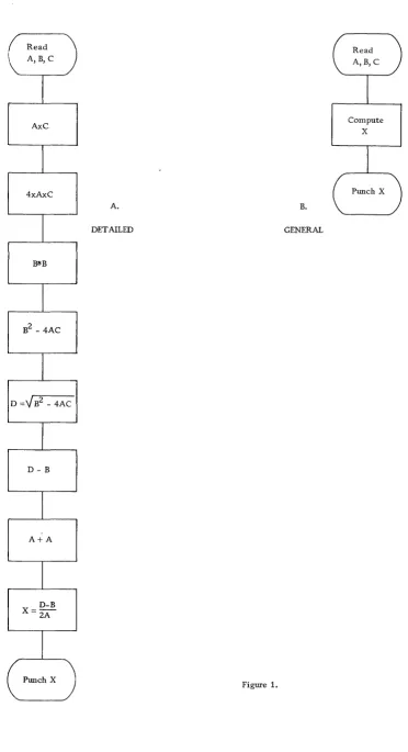
The amount of information put into the block diagram, however, will de-pend upon personal preference, the programming techniques used, and the type of computer to be used. For example, Figure 1 illustrates two ways of block-diagramming the solution of a quadratic equation. The de-tailed diagram shows every step in the computation and is the type that might be used if the programmer were forced to work in machine language. The second diagram shows only the three main steps in the program but is quite sufficient for a programmer using the FORTRAN language.

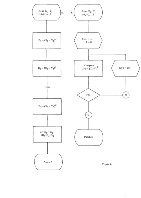
To further illustrate, consider a problem which involves the repetition of the same operation over and over. Let the problem be to create the sum

z =

~

i=l 1 1

This might be block-diagrammed in either of the two ways illustrated in Figure 2.

d

AxC

4xAxC

B'J'B

B2 _ 4AC

D-B

..

A+A

D-B

x=-

A.

DETAILED

Figure 1.

B.

GENERAL

Read Xi' Y_i i=1,2, .. ,S

etc.

z

Punch Z

A. B. Read Xi' Yi

i=1,2, .. ,S

Set i = 1,

Z=O

Compute 2 Z=Z + _{(Xi - Y i )}

Punch Z

J

N

Subscripting

The two diagrams illustrate an important programming concept - that of

looping. Diagram A corresponds to a program in which each (Xi - y_i)2 is computed separately and then all are summed to obtain Z. With only five values of i, this is not too unlikely a method of approaching the prob-lem. But, consider a situation in which i

=

In diagram B, advantage has been taken of the computer's ability to make logical decisions and to modify its own program. Since the number of times the computation is repeated depends only on the value of i (and the presence of successive values ~ and Y

i), this one diagram - and the

program which would be based on it - applies for any value of i.

The algebraically incorrect statement i

=

The purpose of subscripting in mathematics is to simplify notation and at the same time to remove ambiguity of meaning. In computer work the subscript is used in two ways:

1. Spacewise - to specify elements of arrays such as:

Al _{All A12 ·} . AIN

A2 _{A2l A22 ·} . A2N

A3 or _{A3l A32 ·} A3N

This allows reference to elements of an array through simple manipulation of the subscripts - just as in normal mathematical thought.

2. Timewise - to specify the chronological order in which a procedure occurs. For example, in Figure 2, diagram B, the subscript i is used not only to denote which member of the X and Y array is being operated on, but also to indicate how many times the computational step ~ = ~ + (Xo - Yo)2 has been performed. This connotation and use is not so familiar

1 1

Absolute Value

The absolute value becomes important because of the way in which a com-puter makes logical decisions. Comcom-puter decisions are made on the basis of the size of numbers - or, more specifically, upon whether a number is positive, zero or negative. For example, in order to do one of two things dependent upon whether A is (1) less than 500 or (2) equal to or greater than 500, the first thing to do is to subtract 500 from A:

A - 500 = E

Then the decision is based upon the size of E. Specifically, if E is

neg-ative, procedure 1 is done, and if E is positive or zero, procedure 2 is

done.

If the difference represents the error in a procedure (that is, 500 is the

true value and A is the estimate), the absolute value of the error must be less than a prescribed amount e and the test is:

if

IE I -

I

I -

The absolute value must be used, for in general there is no prior knowl-edge of whether the difference A-500 will be positive or negative. All the alternatives must be spelled out to the computer in its program.

In many practical cases the "relative" error is a better measure of the error than the absolute error of a result. The relative error test for the above situation would be stated:

1

°f

~

f500l

-

if

ULJ

I500l

Floating Point Arithmetic

Engineering calculations often involve handling of very large numbers such as Young's modulus, which is 30,000,000 lbs. per sq. in. The common procedure is to write such a number as 3.0 x 107 to facilitate computation.

A similar situation exists in handling very large or very small numbers in a computer. To get away from carrying a great many digits and to eliminate the effort of keeping track of the location of the decimal point for these numbers, a floating point notation is used. A common procedure is to maintain seven or eight most significant digits of a number plus a two-digit "characteristic" to indicate the proper position of the decimal point. The characteristic is developed from the exponent of 10 (assuming use of the decimal system).

For example, the number

- .00000061957533

26

'I

Errors

can be represented as

- . 61957533x10-6

However, this representation requires carrying two signs: one for the exponent and one for the fraction. This is inconvenient for computers which have only one sign associated with a storage location. Therefore, a com-mon practice is to add the exponent to some positive base.

Using a base of 50, the characteristic becomes 50 + (-06) = 44 and the

internal computer representation of the number becomes:

4461957533-A FORTR4461957533-AN programmer need not be concerned with this internal rep-resentation. The number might appear in a FORTRAN program as

- .61957533E-6

There are several sources of errors in computation which deserve con-sideration in any problem.

Initial error: If x is the true value of a data reading and x* is the reading

used in computation (reflecting an error in measurement, perhaps), the

initial error is x - x*.

Rounding error: This type of error results when the less significant digits of a quantity are deleted and a rule of correction is applied to the remain-ing part. For example, pi, 3.14159265 ... , rounded to four decimals, is 3.1416.

Truncation error: To simply chop off at four decimal places for pi, glvlng 3.1415, would result in a truncation error. Another common source of truncation error is in chopping off all terms in an infinite series expansion after a particular term. For example, cutting the series for eX at

eX = 1 + x + x2 + x3

213T

gives truncation error - sometimes called residual error for series approximations.

Propagated error: If x is the true value of a variable and x* the value

used in computation, then f(x) - f(x*) is the propagated error. Errors may build up in computation!

Recursion Formulas

Very often computation of a set of numbers can be simplified by formulas which give one member of the set in terms of other members of the set. An example of this is finding the new coefficients of a polynomial when the

Algorithms

one root of the polynomial equation anxn + _{an- 1 x}n- 1 + ~-2 xn- 2 + •••

a_o = 0, then the original polynomial can be divided by (x - r) to obtain

the reduced polynomial:

a xn- 1 _n + (a 1 _n- + ra ) x n- 2 _n + la _n-2 + r (a _{n - n} 1 + ra >] xn -3 + ••••

x-rJa xn+ a xn- 1 + a xn- 2 + •••

n n-1 n-2

a xn - ra xn- 1

n n

n-1 n-2

(an- 1 + ran> x + lfi-2 x + ••••

(an- 1 + _{ran> xn- 1 - r (an- 1} + ran) xn- 2

[an-2 + r (an- 1 + ran>] xn

-2 + ••••

k k-l

Let: ckx + ck-l x + •.••• + cr + Co

=

be the resulting polynomial (where k = n-1).

Then, equating coefficients gives:

ck-2

=

=

or in general

C _. = a _{. 'I} + rc _{. 1}

1 1+ 1+

This is a recursion formula for c

i. This formula has obvious advantages

for programming the calculation of the new coefficients.

An algorithm is a theorem which may state that a solution to a problem

exists, and/or a procedure for obtaining the solution. The term is fre-quently encountered in computer literature because the form of an equa-tion is often all-important in programming efficiently.

Two examples will be given here:

1. To compute the value of the polynomial

computation is simplified if it is written as

which indicates that the polynomial may be computed by repeating the steps "multiply and add" five times.

2. The square root of a positive real number, A, can be computed by using the algorithm

This example also introduces the idea of iteration. What is meant

by this equation is that to obtain an estimate of A· 5, start with a first

guess xO. Substitute it in the right side of the equation to obtain the

next estimate of A· 5. A few of the steps are:

I

A

xl =-(x_O + - )

2

Xo

x =..!..(x + A )

2 2 1 xl

x3 =.1. _(x2 +A)

2 . x2

=2:.(

x'+_{1 l} 2 x. -_{1 X.}

1

Note that the algorithm states a procedure for solution of the prob-lem, not just one formula evaluation.

Further, note the timewise use of the subscript i; i + 1 indicates a

result dependent upon the previous result subscripted by i.

Taking a value of A (say 25) for which the square root is known, and

performing the indicated operations will make this algorithm clear.

If 2 is used as a starting estimate, then;

Xo = 2

x

=

~

=

1 2 2

I ( 25 ) '"

x = - 7.25 + - - = 5.35

2 2 7.25

x3 =

~

~

There are several ways of deciding the point at which to discontinue the iteration:

a. When differences between successive estimates are less than

some

E

I

I

E

b. When relative differences between successive estimates are

less than some

E

I

1<

E

This makes the choice of

E

c. When relative differences between the function of the estimate and the original function value A are less than some

E

This eliminates the possibility of an erroneous solution in a sit-uation where convergence is slow and is the preferred type of test.

The general statement for this test in finding a value of x which satisfies

f (x) = A

is

In succeeding chapters the problem of solving for values of x which satisfy equations of the form x = f (x) are discussed. Methods a and b remain the same but the test equation corresponding to c above is

Complex Number Calculations

Complex numbers can create some questions of handling and yet are of great importance to electrical and electronic engineers. The following rules handle complex arithmetic:

A. Addition

(a+bi) + (c+di) = (a+c) + (b+d) i

B. Multiplication

(a+bi) (c+di) = (ac-bd) + (ad+bc) i

C. Division

D. Square Root

I If we let u+vi = (a+bi)'2"

squaring both sides gives u 2 + 2uvi - v 2 = a +bi

Equating the real and imaginary parts

(2) 2uv = b orv=

l

2u

then substituting from (2) into (1)

and multiplying through by u2 gives

u4 - au2 - b2 = 0 T

and solving the quadratic gives

u2 =

~ ~ [(~)

(~

nt

Only the positive sign is considered since u is real; thus

(3) u

=[~ +((~)

+(~)2)TJ

t

I

and(4) v =

[-~

(~t i~f

t

r

If a is positive, compute u by (3) and use (2) to find v.

If a is negative, compute v by (4) and use (2) to find u.

E. For a general power of a complex number use

-e-

=

a

and ein

'-9;

ne-then (a+bi)n = rn (cos nB- + i sin n-9-)

Transformations and Identities

Exercises

For example, assume in a particular problem that the value for the tan-gent of an angle is given:

tan

-e-

and that cos

-e-

~ = tan -1 A and then compute the cos

-e-.

immediately be computed as

cos

-e-

~r""I=+=A=2i::-

~A

saving the evaluation of two trigonometric functions.

A useful transformation in computing is the logarithmic transformation.

Suppose we have an exponential function y = k xa. If we take the natural

log of both sides, we have

log y = a log x + log k

thus reducing an exponential relationship between x and y to a linear rela-tionship between the transformed variables log x and log y.

Most of the mathematical techniques which have been outlined here are quite familiar to the average engineer. However, they are given this emphasis because recognition of their use in particular situations can greatly simplify solution of computer problems.

1. For the set of tabular data shown, construct the difference table to determine to what degree of x is y dependent.

x y

0 0

1 3

2 18

3 57

4 132

5 255

6 438

2. Divide 8 + 12i by 3 + 2i.

3. U sing the iteration formula for finding the square root of a number, find the square root of 12 accurate to 7 places (the absolute difference

between two successive estimates of

ill

*4. Using only the functions SINF(X), C<pSF(X) , ATANF(X) , EXPF(X) , L<\>GF(X) and SQRTF(X) , write the FORTRAN statement for computing all trigonometric, inverse trigonometric and hyperbolic functions.

5. Construct a block diagram chart to show the logic of computing the value of the polynomial

where the values of the coefficients aI' a , _____ a

6 are to be read into the computer and the value of f

tX)

*6. Repeat 5 and generalize the block diagram to show the logic of han-dling any degree polynomial. That is, block-diagram the computation of f (x), where

7. Write a FORTRAN program for exercise 6.

SECTION IV: PRINCIPLES OF ITERATION

Arithmetic, Mathematics and the Computer

Although arithmetic is one class of mathematical operation, for purposes of clarity it is best to differentiate arithmetic operations from the other mathematical operations in discussing computers. Arithmetic is performed when any of the operations of addition, subtraction, multiplication and division are applied to a pair of numbers. Other mathematical operations are performed when one of a variety of operations such as algebraic sub-stitution, integration, differentiation, expansion to series representation, etc., is applied to one or more symbols. In essence arithmetic deals with numbers while mathematics is the manipulation of symbols.

Computers are designed to efficiently perform all the arithmetic opera-tions. Most computers can also handle in a limited way the alphabetic and some special characters which might be used as symbols (as is obvious from the use of the computer to translate FORTRAN programs).

The computer, as designed, cannot do original mathematics. However, once the mathematics of a problem are accomplished, the computer is most useful in obtaining the required numerical values by performing the necessary arithmetic operations.

In addition, once a particular mathematical problem has been properly solved and the program for arithmetic evalu,ation on a computer has been completed, all similar problems, differing only in data values, can be henceforth evaluated by the one program. Two examples will illustrate these facts:

A. Given the two simultaneous equations

find values of x and x which satisfy these equations when

1 2

a

11=2, aI2=2, a21=3, a22=4, b1=5, b2=6

To solve this problem we have distinct mathematical and arithmetic steps.

Mathematically:

Algebraically using (1) write Xl as a function of x₂

b - a x x = f (x) = 1 12 2

1 1 2 a

11

(3)

Substitute this function fl (x2) in the second equation to obtain an equa-tion in x

This equation may then be treated algebraically to give x

2 as a function of the coefficients only

X2

~

(b

b

all all

Arithmetically:

Substitute the values given for the coefficients in equation (5) to deter-mine x₂

==-1.5

Use this result in equation (3) to find a value for xl

x = 5 - 2( -1. 5) = 4

1 2

The computer solution to this problem considers only the arithmetic op-erations implied by equations (3) and (5). A FORTRAN program to eval-uate these two equations is shown in Figure 3 .

. EC FOR COMMENT

+s~=~ ~

1 5 67 FORTRAN STATEMENT 72

4 R E.A /) 1 (), K, A , 8,

X(:i) := (B,(2.)-A(,Z,l)*8(1)I.A(J,l»I.(A(2,Z)-A(,Z,l)-ifA(1.Z)I.A(J,l))

X ( I ) .:: (8(1)-)«(2)*A(,1 2»/A(1,1

PIl I N,7, /l. b, K

,x

Figure 3.

NOTE the following items of interest concerning this program:

1. Only the solution equations have been programmed. The original equations are not of interest to the computer since the mathematics must be performed before using the computer.

2. Equations (3) and (5) are programmed in their symbolic form and actual values for the coefficients are read into the computer before

compu-tation takes place. By programming in this way the computer can now

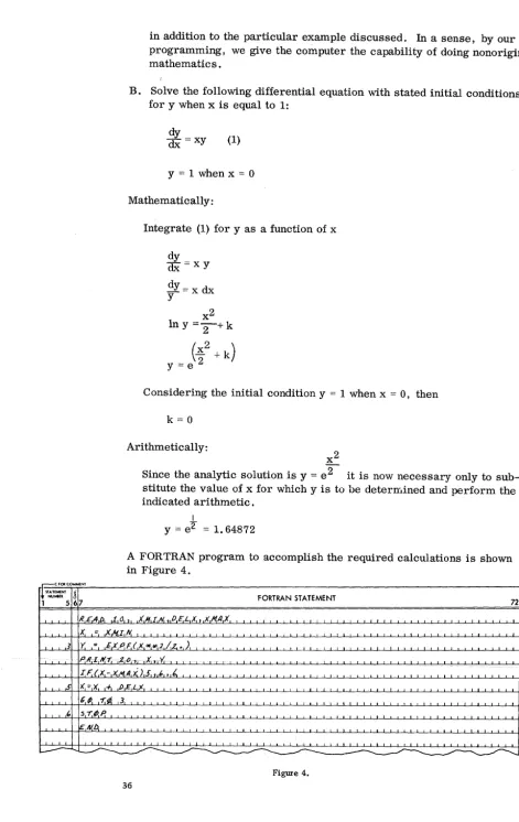
in addition to the particular example discussed. In a sense, by our programming, we give the computer the capability of doing nonoriginal mathematic s .

B. Solve the following differential equation with stated initial conditions for y when x is equal to 1:

: = xy (1)

y

=

=

Mathematically:

Integrate (1) for y as a function of x

dy

dx =x Y

dy = x dx

Y

x2

lny

=2+

(~2

+

k)

y:::e

Considering the initial condition y ::: 1 when x ::: 0, then

Arithmetically:

x 2

Since the analytic solution is y ::: e

2

I

Y ::: e2 ::: 1.64872

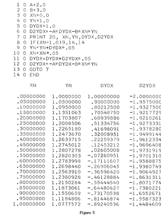
A FORTRAN program to accomplish the required calculations is shown in Figure 4.

'EC FOR COMMENT

.s~=:r ~

1 567 FORTRAN STATEMENT 72

~E.AD to, XHIN.,D£.£X,XM.AX

x

3 Y. ~ kXP.F(X*~2/' . )

IF(J<.-x,M./I X.) S, 6. 6.

NOTE the following:

1. Again only the analytic solution is programmed.

2. The program is written so as to allow many values of y to be com-puted over any range in x.

Nume rical Analysis

The two problems chosen happen to be of types for which the mathematical analysis is well defined. The variables in que stion may be equated to

functions of the known quantities - analogous to the formula y = f (x, z) as

discussed in the first chapter.

Various analytic techniques successfully handle a large class of the math-ematical problems which arise in the description of the physical world. However, a vastly larger number of mathematical problems are not sub-ject to the normal analytic procedures of algebra, analytic geometry, or the calculus.

For the theoretical mathematician or physicist it may be sufficient, when meeting these problems, to be able to show that one or more approxima-tions will allow an analytic solution of the problem to any desired degree of accuracy.

The engineer, on the other hand, must have a solution from which accurate

numerical results can be obtained if the theory is to be of value. These

results must be obtained at a reasonable expense of time and effort. A mathematician may be content to know that a series will converge. An engineer must be concerned with the number of terms in the series re-quired for a given accuracy.

Numerical analysis provides techniques for finding concrete numerical results for mathematical problems of the type under discussion. This manual describes many physical problems which require numerical analy-sis. Some of the simpler analysis techniques are discussed. The reader is referred to the many excellent texts available on numerical analysis for an adequate discussion of particular analysis theory.

Algebraic Equation

T 1 cos B- - T 2 cos <I> = 0

T 1 sin

-e-

T 1 and T 2 are readily solved for specified values of

-e- ,

Consider a set of equations similar to A but containing a simple nonlinearity:

(1)

(2)

The previous algebraic steps would give:

a12 b

x = - - x 2 + 1

1 all all

(3)

and:

a 1b1 x 2 / a a

x = (b - _2_ - a e ) (- 21 12)

2 2 a 22 a

11 11

or with appropriate substitutions for (4)

bX2

x

=

2

(4)

This gives an equation in x₂ only, but from the equation it is impossible to directly evaluate x

2. One approach is to expand ebx2 to several terms of its series:

Equations of Calculus

Similarly the differential equation of example B has an analytic solution. However, the differential equation

has no corresponding analytic solution. To find values of y for corre-sponding values of x, a numerical approach is necessary. Likewise, many integrals may be obtained only by numerical approximations. Again, some simple techniques will be given for handling this type of problem.

Iteration Type Problems

There are three principal reasons for the use of iteration with computer handling of engineering problems.

1. The mathematical statement of the physical problem requires an itera-tion approach for evaluating one or more of the variables.

The chart below shows exalllples of four types of mathematical problem statements.

Single Equations

<t> = tan<p-K

Multiple Equations

RHe - RH m= _ _ _ _ _

Direct Iteration Sufficient

Numerical Techniques L = A sin (900 - B - ~ -0() - (R-E) Required

2. Many designs are to be evaluated in a search for the best design, that is, optimization of design. Often this problem can be reduced to the previous problem by selection of an appropriately expressed mathemat-ical criterion of what is optional.

3. The mathematical expression for the physical problem is to be

eval-uated for many values of one or more known parameters - such as

time, in a problem of motion, or degree of rotation, in a geometry problem.

A. One problem which illustrates iteration is the solution of an equation which arises frequently in absorption problems of optics, electric fields and nuclear engineering:

where a and b are constants.

This cannot be solved explicitly for x, so the following iteration pro-cedure is used:

1. Make a guess at x.

2. Use this in right-hand side of equation (1) to give a new value for x.

3. Call this new value of x the next guess.

4. Repeat steps 2 and 3 until two successive guesses either agree or differ by an amount less than the allowable error.

A FORTRAN program to solve such a problem, where

x = O. 2eO• 5x

is as follows:

READ 10, A, B, X

1 PRINT,X

2 XNEW=O. 2*EXPF(0. 5*X)

TES T=ABSF (X -XN EW)

IF(TEST-. 00005)4, 4,3

3 X=XNEW

GO TO 1

4 PRINT, XNEW

END

Read values for A, Band initial estimate of x (1. 0).

Print estimate of x.

FORTRAN arithmetic state-ment of equation to be solved.

Find absolute value of dif-ference in last two estimates.

If difference is less than or equal to .00005, go to step 4. Otherwise, go to step 3.

Store new estimate of x.

Return to step 1 and repeat.

Print last estimate of x.

End of progr am •

If this were translated into machine language and the resulting program run on a computer, the successive estimates of x would be:

X 1.000000

The last value in the list satisfies the requirement tha