the smile. We apply the SABR model to USD interest rate options, and find good agreement between the theoretical and observed smiles.
Key words. smiles, skew, dynamic hedging, stochastic vols, volga, vanna
1 Introduction
European options are often priced and hedged using Black’s model, or, equivalently, the Black-Scholes model. In Black’s model there is a one-to-one relation between the price of a European option and the volatility parameter σB. Consequently, option prices are often quoted by stating the implied volatilityσB, the unique value of the volatility which yields the option’s dollar price when used in Black’s model. In theory, the volatility
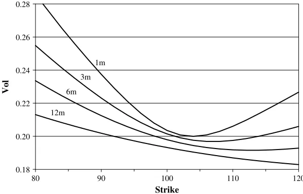
σB in Black’s model is a constant. In practice, options with different strikes Krequire different volatilities σBto match their market prices. See figure 1. Handling these market skews and smilescorrectly is critical to fixed income and foreign exchange desks, since these desks usually have large exposures across a wide range of strikes. Yet the inherent contra-diction of using different volatilities for different options makes it diffi-cult to successfully manage these risks using Black’s model.
Patrick S. Hagan
*
,
Deep Kumar
†
,
Andrew S. Lesniewski
‡
,
and
Diana E. Woodward
§
Managing
Smile Risk
AbstractMarket smiles and skews are usually managed by using local volatility models a laDupire. We discover that the dynamics of the market smile pre-dicted by local vol models is opposite of observed market behavior: when the price of the underlying decreases, local vol models predict that the smile shifts to higher prices; when the price increases, these models pre-dict that the smile shifts to lower prices. Due to this contrapre-diction between model and market, delta and vega hedges derived from the model can be unstable and may perform worse than naive Black-Scholes’ hedges.
To eliminate this problem, we derive the SABR model, a stochastic volatility model in which the forward value satisfies
dFˆ= ˆaFˆβdW
1
daˆ=νa dWˆ 2
and the forward Fˆand volatility aˆare correlated: dW1dW2=ρdt. We use
singular perturbation techniques to obtain the prices of European options under the SABR model, and from these prices we obtain explicit, closed-form algebraic formulas for the implied volatility as functions of today’s forward price f= ˆF(0)and the strike K. These formulas immedi-ately yield the market price, the market risks, including vannaand volga risks, and show that the SABR model captures the correct dynamics of
*[email protected]; Bear-Stearns Inc, 383 Madison Ave, New York, NY 10179 †BNP Paribas; 787 Seventh Avenue; New York NY 10019
‡BNP Paribas; 787 Seventh Avenue; New York NY 10019
The development of local volatility modelsby Dupire [2], [3] and Derman-Kani [4], [5] was a major advance in handling smiles and skews. Local volatility models are self-consistent, arbitrage-free, and can be calibrated to precisely match observed market smiles and skews. Currently these mod-els are the most popular way of managing smile and skew risk. However, as we shall discover in section 2, the dynamicbehavior of smiles and skews predicted by local vol models is exactly oppositethe behavior observed in the marketplace: when the price of the underlying asset decreases, local vol models predict that the smile shifts to higherprices; when the price increas-es, these models predict that the smile shifts to lowerprices. In reality, asset prices and market smiles move in the samedirection. This contradiction between the model and the marketplace tends to de-stabilize the delta and vega hedges derived from local volatility models, and often these hedges perform worse than the naive Black-Scholes’ hedges.
To resolve this problem, we derive the SABR model, a stochastic volatility model in which the asset price and volatility are correlated. Singular perturbation techniques are used to obtain the prices of European options under the SABR model, and from these prices we obtain a closed-form algebraic formula for the implied volatility as a function of today’s forward price fand the strike K. This closed-form for-mula for the implied volatility allows the market price and the market risks, including vannaand volgarisks, to be obtained immediately from Black’s formula. It also provides good, and sometimes spectacular, fits to the implied volatility curves observed in the marketplace. See Figure 1.1. More importantly, the formula shows that the SABR model captures the correct dynamics of the smile, and thus yields stable hedges.
2 Reprise
Consider a European call option on an asset A with exercise date tex,
settle-ment date tset, and strike K. If the holder exercises the option on tex, then on
the settlement date tset he receives the underlying asset Aand pays the
strike K. To derive the value of the option, define Fˆ(t)to be the forward price of the asset for a forward contract that matures on the settlement date tset, and define f= ˆF(0)to be today’s forward price. Also let D(t)be
the discount factorfor date t; that is, let D(t)be the value today of $1 to be delivered on date t. Martingale pricing theory [6-9] asserts that under the “usual conditions,” there is a measure, known as the forward measure, under which the value of a European option can be written as the expect-ed value of the payoff. The value of a call options is
Vcall =D(tset)E
[Fˆ(tex)−K]+|F0
, (2.1a)
and the value of the corresponding European put is
Vput=D(tset)E
[K− ˆF(tex)]+|F0
≡Vcall+D(tset)[K−f].
(2.1b)
Here the expectation Eis over the forward measure, and “|F0” can be
inter-pretted as “given all information available at t=0.” Martingale pricing the-ory [6-9] also shows that the forward price Fˆ(t)is a Martingale under this measure, so the Martingale representation theorem shows that Fˆ(t)obeys
dFˆ=C(t,∗)dW, Fˆ(0)=f, (2.1c) for some coefficient C(t,∗), where dWis Brownian motion in this meas-ure. The coefficient C(t,∗)may be deterministic or random, and may depend on any information that can be resolved by time t. This is as far as the fundamental theory of arbitrage free pricing goes. In particular, one cannot determine the coefficient C(t,∗)on purely theoretical grounds. Instead one must postulate a mathematical modelfor C(t,∗).
European swaptions fit within an indentical framework. Consider a European swaption with exercise date tex and fixed rate (strike) Rfix. Let
Rs(t) be the swaption’s forward swap rate as seen at date t, and let R0= ˆRs(0)be the forward swap rate as seen today. In [9] Jamshidean shows
that one can choose a measure in which the value of a payer swaption is Vpay=L0E
[Rˆs(tex)−Rfix]+|F0
, (2.2a)
and the value of a receiver swaption is
Vrec=L0E
[Rfix− ˆRs(tex)]+|F0
≡Vpay+L0[Rfix−R0].
(2.2b)
Here the level L0is today’s value of the annuity, which is a known
quanti-ty, and Eis the expectation over thelevel measure of Jamshidean [9]. In Appendix A it is also shown that the PV01 of the forward swap; like the
W
M99 Eurodollar option
5 10 15 20 25 30
92.0 93.0 94.0 95.0 96.0 97.0
Strike
Vol (%)
discount factor rate Rˆs(t)is a Martingale in this measure, so once again dRˆs=C(t,∗)dW, Rˆs(0)=R0, (2.2c)
where dWis Brownian motion. As before, the coefficient C(t,∗)may be deterministic or random, and cannot be determined from fundamental theory. Apart from notation, this is identical to the framework provided by equations (2.1a–2.1c) for European calls and puts. Caplets and floor-lets can also be included in this picture, since they are just one period payer and receiver swaptions. For the remainder of the paper, we adopt the notation of (2.1a–2.1c) for general European options.
2.1 Black’s model and implied volatilities. To go any further requires postulating a model for the coefficient C(t,∗). In [10], Black pos-tulated that the coefficient C(t,∗) is σBFˆ(t), where the volatiltyσB is a constant. The forward price Fˆ(t)is then geometric Brownian motion:
dFˆ=σBFˆ(t)dW, Fˆ(0)=f. (2.3) Evaluating the expected values in (2.1a, 2.1b) under this model then yields Black’s formula,
Vcall=D(tset){fN(d1)−KN(d2)}, (2.4a)
Vput =Vcall+D(tset)[K−f], (2.4b)
where
d1,2=
logf/K±1 2σ
2
Btex σB√tex
, (2.4c)
for the price of European calls and puts, as is well-known [10], [11], [12]. All parameters in Black’s formula are easily observed, except for the volatility σB. An option’s implied volatilityis the value of σBthat needs to be used in Black’s formula so that this formula matches the market price of the option. Since the call (and put) prices in (2.4a – 2.4c) are increasing functions of σB, the volatility σBimplied by the market price of an option is unique. Indeed, in many markets it is standard practice to quote prices in terms of the implied volatility σB; the option’s dollar price is then recovered by substituting the agreed upon σBinto Black’s formula.
The derivation of Black’s formula presumes that the volatility σBis a constant for each underlying asset A. However, the implied volatility needed to match market prices nearly always varies with both the strike K and the time-to-exercise tex. See Figure 2.1. Changing the volatility σB
means that a differentmodel is being used for the underlying asset for each K and tex. This causes several problems managing large books of
options.
The first problem is pricing exotics. Suppose one needs to price a call option with strike K1 which has, say, a down-and-out knock-out at
K2<K1. Should we use the implied volatility at the call’s strike K1, the
implied volatility at the barrier K2, or some combination of the two to
price this option? Clearly, this option cannot be priced without a single, self-consistent, model that works for all strikes without “adjustments.”
The second problem is hedging. Since differentmodels are being used for differentstrikes, it is not clear that the delta and vega risks calculated at one strike are consistent with the same risks calculated at other strikes. For example, suppose that our 1 month option book is long high strike options with a total risk of +$1MM, and is long low strike options with a
of −$1MM. Is our is our option book really -neutral, or do we have residual delta risk that needs to be hedged? Since different models are used at each strike, it is not clear that the risks offset each other. Consolidating vega risk raises similar concerns. Should we assume parallel or proportional shifts in volatility to calculate the total vega risk of our book? More explicitly, suppose that σB is 20% at K=100 and 24% at K=90, as shown for the 1m options in Figure 2.1 Should we calculate vega by bumping σBby, say, 0.2% for both options? Or by bumping σBby 0.2% for the first option and by 0.24% for the second option? These questions are critical to effective book management, since this requires consolidating the delta and vega risks of alloptions on a given asset before hedging, so that only the net exposure of the book is hedged. Clearly one cannot answer these questions without a model that works for all strikes K.
The third problem concerns evolution of the implied volatility curve
σB(K). Since the implied volatility σBdepends on the strike K, it is likely to also depend on the current value fof the forward price: σB=σB(f,K). In this case there would be systematic changes in σBas the forward price fof the underlying changes See Figure 2.1. Some of the vega risks of Black’s model would actually be due to changes in the price of the underlying asset, and should be hedged more properly (and cheaply) as delta risks.
0.18 0.20 0.22 0.24 0.26 0.28
80 90 100 110 120
Strike
Vol
1m 3m 6m
12m
^
2.2 Local volatility models. An apparent solution to these problems is provided by the local volatility model of Dupire [2], which is also attrib-uted to Derman [4], [5]. In an insightful work, Dupire essentially argued that Black was to bold in setting the coefficient C(t,∗)to σBF. Instead oneˆ should only assume that Cis Markovian: C=C(t,Fˆ). Re-writing C(t,Fˆ)as
σloc(t,Fˆ)Fˆthen yields the “local volatility model,” where the forward price of the asset is
dFˆ=σloc(t,Fˆ)FdWˆ , Fˆ(0)=f, (2.5a) in the forward measure. Dupire argued that instead of theorizing about the unknown local volatility function σloc(t,Fˆ), one should obtain
σloc(t,Fˆ)directly from the marketplace by “calibrating” the local volatili-ty model to market prices of liquid European options.
In calibration, one starts with a given local volatility function
σloc(t,Fˆ), and evaluates Vcall=D(tset)E
[Fˆ(tex)−K]+| ˆF(0)=f,
(2.5b)
≡Vput+D(tset)(f−K) (2.5c)
to obtain the theoretical prices of the options; one then varies the local volatility function σloc(t,Fˆ)until these theoretical prices match the actu-al market prices of the option for each strike Kand exercise date tex. In
practice liquid markets usually exist only for options with specific exer-cise dates t1
ex,tex2,tex3, . . .; for example, for 1m, 2m, 3m, 6m, and 12m from
today. Commonly the local vols σloc(t,Fˆ)are taken to be piecewise con-stant in time:
σloc(t,Fˆ)=σloc(1)(Fˆ) fort<tez1,
σloc(t,Fˆ)=σloc(j)(Fˆ) fortexj−1<t<tezj j=2,3, . . .J
σloc(t,Fˆ)=σloc(J)(Fˆ) fort>tezJ
(2.6)
One first calibrates σloc(1)(Fˆ)to reproduce the option prices at t1
exfor all
strikes K, then calibrates σloc(2)(Fˆ)to reproduce the option prices at t2
ex, for
all K, and so forth. This calibration process can be greatly simplified by using the results in [13] and [14]. There we solve to obtain the prices of European options under the local volatility model (2.5a–2.5c), and from these prices we obtain explicit algebraic formulas for the implied volatil-ity of the local vol models.
Once σloc(t,Fˆ) has been obtained by calibration, the local volatility model is a single, self-consistent model which correctly reproduces the market prices of calls (and puts) for all strikes Kand exercise dates tex
without “adjustment.” Prices of exotic options can now be calculated from this model without ambiguity. This model yields consistent delta
and vega risks for all options, so these risks can be consolidated across strikes. Finally, perturbing fand re-calculating the option prices enables one to determine how the implied volatilites change with changes in the underlying asset price. Thus, the local volatility model thus provides a method of pricing and hedging options in the presence of market smiles and skews. It is perhaps the most popular method of managing exotic equity and foreign exchange options. Unfortunately, the local volatility model predicts the wrong dynamicsof the implied volatility curve, which leads to inaccruate and often unstable hedges.
To illustrate the problem, consider the special case in which the local vol is a function of Fˆonly:
dFˆ=σloc(Fˆ)FdWˆ , Fˆ(0)=f. (2.7)
In [13] and [14] singular perturbation methods were used to analyze this model. There it was found that European call and put prices are given by Black’s formula (2.4a-2.4c) with the implied volatility
σB(K,f)=σloc
1
2[f+K] 1+ 1 24
σloc(1 2[f+K])
σloc(1 2[f+K])
(f−K)2+ · · ·.(2.8)
On the right hand side, the first term dominates the solution and the second term provides a much smaller correction The omitted terms are very small, usually less than 1% of the first term.
The behavior of local volatility models can be largely understood by examining the first term in (2.8). The implied volatility depends on both the strike Kand the current forward price f.So supppose that today the forward price is f0 and the implied volatility curve seen in the
market-place is σ0
B(K). Calibrating the model to the market clearly requires
choosing the local volatility to be
σloc(Fˆ)=σ0
B(2Fˆ−f0){1+ · · ·}. (2.9)
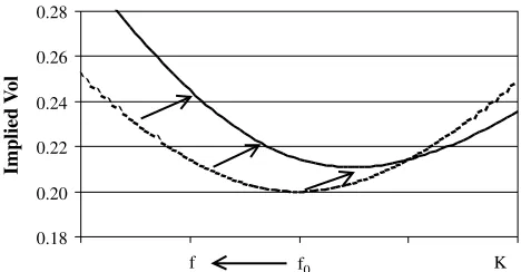
Now that the model is calibrated, let us examine its predictions. Suppose that the forward value changes from f0 to some new value f. From (2.8),
(2.9) we see that the model predicts that the new implied volatility curve is
σB(K,f)=σ0
B(K+f−f0){1+ · · ·} (2.10)
for an option with strike K, given that the current value of the forward price is f. In particular, if the forward price f0 increasesto f, the implied
volatility curve moves to the left; if f0decreasesto f, the implied volatility
To demonstrate the problem concretely, suppose that today’s implied volatility is a perfect smile
σ0
B(K)=α+β[K−f0]2 (2.11a)
around today’s forward price f0. Then equation (2.8) implies that the
local volatility is
σloc(Fˆ)=α+3β(Fˆ−f0 2
)+ · · ·. (2.11b)
As the forward price fevolves away from f0due to normal market
fluctu-ations, equation (2.8) predicts that the implied volatility is
σB(K,f)=α+βK−3 2f0−12f
2
+3
4β (f−f0) 2
+ · · ·. (2.11c)
The implied volatility curve not only moves in the opposite direction as the underlying, but the curve also shifts upward regardless of whether f increases or decreases. Exact results are illustrated in Figures 2.2 – 2.4. There we assumed that the local volatility σloc(Fˆ)was given by (2.11b), and used finite difference methods to obtain essentially exact values for the option prices, and thus implied volatilites.
Hedges calculated from the local volatility model are wrong. To see this, let BS(f,K, σB,tex) be Black’s formula (2.4a–2.4c) for, say, a call
option. Under the local volatility model, the value of a call option is given by Black’s formula
Vcall=BS(f,K, σB(K,f),tex) (2.12a)
with the volatility σB(K,f)given by (2.8). Differentiating with respect to f yields the risk
≡∂Vcall
∂f =
∂BS
∂f +
∂BS
∂σB
∂σB(K,f)
∂f . (2.12b)
predicted by the local volatility model. The first term is clearly the risk one would calculate from Black’s model using the implied volatility from the market. The second term is the local volatility model’s correction to the risk, which consists of the Black vega risk multiplied by the predict-edchange in σBdue to changes in the underlying forward price f. In real markets the implied volatily moves in the oppositedirection as the direc-tion predicted by the model. Therefore, the correcdirec-tion term needed for real markets should have theopposite signas the correction predicted by the local volatility model. The original Black model yields more accurate hedges than the local volatility model, even though the local vol model is self-consistent across strikes and Black’s model is inconsistent.
Local volatility models are also peculiar theoretically. Using any func-tion for the local volatility σloc(t,Fˆ)exceptfor a power law,
C(t,∗)=α(t)Fˆβ, (2.13)
σloc(t,Fˆ)=α(t)Fˆβ/Fˆ=α(t) /Fˆ1−β, (2.14)
0.18 0.20 0.22 0.24 0.26 0.28
Implied V
o
l
K f0
Fig. 2.2 Exact implied volatility σB(K,f0)(solid line) obtained from the local volatility σloc(Fˆ)(dashed line):
0.18 0.20 0.22 0.24 0.26 0.28
Implied V
o
l
K f0
f
Fig. 2.3 Implied volatility σB(K,f)if the forward price decreasesfrom f0to f(solid line).
0.18 0.20 0.22 0.24 0.26 0.28
Implied V
o
l
f0 f K
^
introduces an intrinsic “length scale” for the forward price Fˆinto the model. That is, the model becomes inhomogeneous in the forward price
ˆ
F. Although intrinsic length scales are theoretically possible, it is diffi-cult to understand the financial origin and meaning of these scales [15], and one naturally wonders whether such scales should be introduced into a model without specific theoretical justification.
2.3 The SABR model. The failure of the local volatility model means that we cannot use a Markovian model based on a single Brownian motion to manage our smile risk. Instead of making the model non-Markovian, or basing it on non-Brownian motion, we choose to develop a two factor model. To select the second factor, we note that most markets experience both relatively quiescent and relatively chaotic periods. This suggests that volatility is not constant, but is itself a random function of time. Respecting the preceding discusion, we choose the unknown coef-ficient C(t,∗) to be αˆFˆβ, where the “volatility” αˆ is itself a stochastic
process. Choosing the simplest reasonable process for αˆ now yields the “stochastic-αβρ model,” which has become known as the SABR model. In this model, the forward price and volatility are
dFˆ= ˆαFˆβdW
1, Fˆ(0)=f (2.15a)
dαˆ =ναˆdW2, α(ˆ 0)=α (2.15b)
under the forward measure, where the two processes are correlated by: dW1dW2=ρdt. (2.15c)
Many other stochastic volatility models have been proposed, for example [16], [17], [18], [19]. However, the SABR model has the virtue of being the simplest stochastic volatility model which is homogenous in Fˆand αˆ. We shall find that the SABR model can be used to accurately fit the implied volatility curves observed in the marketplace for any single exercise date tex. More importantly, it predicts the correct dynamics of the implied
volatility curves. This makes the SABR model an effective means to man-age the smile risk in markets where each asset only has a single exercise date; these markets include the swaption and caplet/floorlet markets.
As written, the SABR model may or may not fit the observed volatility surfaceof an asset which has European options at several different exer-cise dates; such markets include foreign exchange options and most equity options. Fitting volatility surfaces requires the dynamic SABR model which is discussed in an Appendix.
It has been claimed by many authors that stochastic volatility mod-els are modmod-els of incomplete markets, because the stochastic volatility risk cannot be hedged. This is not true. It is true that the risk to changes in αˆ(the vega risk) cannot be hedged by buying or selling the underlying asset. However, vega risk can be hedged by buying or selling options on the asset in exactly the same way that -hedging is used to neutralize the risks to changes in the price F. In practice, vega risks areˆ
hedged by buying and selling options as a matter of routine, so whether the market would be complete if these risks were not hedged is a moot question.
The SABR model (2.15a–2.15c) is analyzed in Appendix B. There sin-gular perturbation techniques are used to obtain the prices of European options. From these prices, the options’ implied volatility σB(K,f)is then obtained. The upshot of this analysis is that under the SABR model, the price of European options is given by Black’s formula,
Vcall=D(tset){fN(d1)−KN(d2)}, (2.16a)
Vput =Vcall+D(tset)[K−.f], (2.16a)
with
d1,2=
logf/K±1 2σ
2
Btex σB√tex
, (2.16c)
where the implied volatility σB(f,K)is given by
σB(K,f)
= α
(f K)(1−β ) /21+(1−β )2
24 log 2
f/K+(11920−β )4log4f/K+ · · ··
z x(z)
·
1+
(1−β )2
24
α2
(f K)1−β +
1 4
ρβνα (f K)(1−β ) /2 +
2−3ρ2
24 ν
2
tex+ · · ·.
(2.17a) Here
z= ν
α(f K)
(1−β ) /2
logf/K, (2.17b) and x(z)is defined by
x(z)=log 1−2ρz+z
2+z−ρ
1−ρ
. (2.17c)
For the special case of at-the-money options, options struck at K=f, this formula reduces to
σATM =σB(f,f)= α
f(1−β )
1+
(1−β )2
24
α2
f2−2β
+1
4
ρβαν
f(1−β ) +
2−3ρ2
24 ν
2
tex+ · · ·.
These formulas are the main result of this paper. Although it appears formidable, the formula is explicit and only involves elementary trigno-metric functions. Implementing the SABR model for vanilla options is very easy, since once this formula is programmed, we just need to send the options to a Black pricer. In the next section we examine the qualitative behavior of this formula, and how it can be used to managing smile risk.
The complexity of the formula is needed for accurate pricing. Omitting the last line of (2.17a), for example, can result in a relative error that exceeds three per cent in extreme cases. Although this error term seems small, it is large enough to be required for accurate pricing. The omitted terms “+ · · ·” are much, muchsmaller. Indeed, even though we have derived more accurate expressions by continuing the perturbation expansion to higher order, (2.17a – 2.17c) is the formula we use to value and hedge our vanilla swaptions, caps, and floors. We have not imple-mented the higher order results, believing that the increased precision of the higher order results is superfluous.
There are two special cases of note: β=1, representing a stochastic log normal model), and β=0, representing a stochastic normal model. The implied volatility for these special cases is obtained in the last sec-tion of Appendix B.
3 Managing Smile Risk
The complexity of the above formula for σB(K,f)obscures the qualita-tive behavior of the SABR model. To make the model’s phenomenology and dynamics more transparent, note that formula (2.17a – 2.17c) can be approximated as
σB(K,f)= α
f1−β
1−1
2(1−β−ρλ )logK/f
+ 1
12
(1−β)2+(
2−3ρ2
) λ2log2K/f+ · · ·,
(3.1a)
provided that the strike Kis not too far from the current forward f. Here the ratio
λ= ν
αf
1−β (3.1b)
measures the strength ν of the volatility of volatility (the “volvol”) com-pared to the local volatility α/f1−βat the current forward. Although
equa-tions (3.1a–3.1b) should not be used to price real deals, they are accurate enough to depict the qualitative behavior of the SABR model faithfully.
As f varies during normal trading, the curve that the ATM volatility
σB(f,f)traces is known as the backbone, while the smileand skewrefer to the implied volatility σB(K,f)as a function of strike Kfor a fixed f. That is, the market smile/skew gives a snapshot of the market prices for dif-ferent strikes K at a given instance, when the forward fhas a specific price. Figures 3.1 and 3.2. show the dynamics of the smile/skew predicted by the SABR model.
Let us now consider the implied volatility σB(K,f)in detail. The first factor α/f1−β in (3.1a( is the implied volatility for at-the-money (ATM)
options, options whose strike Kequals the current forward f.So the back-bone traversed by ATM options is essentially σB(f,f)=α/f1−β for the
SABR model. The backbone is almost entirely determined by the expo-nent β, with the exponent β=0(a stochastic Gaussian model) giving a steeply downward sloping backbone, and the exponent β=1giving a nearly flat backbone.
The second term −1
2(1−β−ρλ )logK/f represents the skew, the
slope of the implied volatility with respect to the strike K. The
−1
2(1−β )logK/fpart is the beta skew, which is downward sloping since
0≤β≤1. It arises because the “local volatility” αˆFˆβ/Fˆ1= ˆα/Fˆ1−β is a
decreasing function of the forward price. The second part 1
2ρλlogK/fis
the vannaskew, the skew caused by the correlation between the volatility and the asset price. Typically the volatility and asset price are negatively correlated, so on average, the volatility αwould decrease (increase) when the forward fincreases (decreases). It thus seems unsurprising that a negative correlation ρcauses a downward sloping vanna skew.
It is interesting to compare the skew to the slope of the backbone. As f changes to fthe ATM vol changes to
8% 10% 12% 14% 16% 18% 20% 22%
4% 6% 8% 10% 12%
Implied vol
β= 0
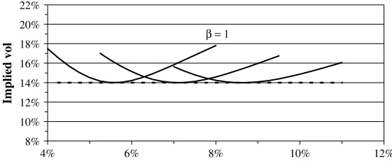
Fig. 3.1 Backbone and smiles for β=0. As the forward fvaries, the implied volatiliity σB(f,f)of ATM options traverses the backbone (dashed curve). Shown are the smiles σB(K,f)for three different values of the forward. Volatility data from 1 into 1 swaption on 4/28/00, courtesy of Cantor-Fitzgerald.
β= 1
8% 10% 12% 14% 16% 18% 20% 22%
4% 6% 8% 10% 12%
Implied vol
^
σB(f,f )= α
f1−β
1−(1−β )f −f
f + · · ·
. (3.2a)
Near K=f, the βcomponent of skew expands as
σB(K,f)= α
f1−β
1−1 2(1−β )
K−f f + · · ·
, (3.2b)
so the slope of the backbone σB(f,f)is twice as steep as the slope of rthe smile σB(K,f)due to the β-component of the skew.
The last term in (3.1a) also contains two parts. The first part
1 12(1−β )
2log2
K/fappears to be a smile (quadratic) term, but it is domi-nated by the downward sloping beta skew, and, at reasonable strikes K, it just modifies this skew somewhat. The second part 1
12(2−3ρ 2)
λ2log2
K/fis the smile induced by the volga(vol-gamma) effect. Physically this smile arises because of “adverse selection”: unusually large move-ments of the forward Fˆhappen more often when the volatility α increas-es, and less often when αdecreases, so strikes Kfar from the money rep-resent, on average, high volatility environments.
3.1 Fitting market data. The exponent β and correlation ρ affect the volatility smile in similar ways. They both cause a downward slop-ing skew in σB(K,f)as the strike K varies. From a single market snap-shot of σB(K,f)as a function of Kat a given f, it is difficult to distin-guish between the two parameters. This is demonstrated by figure 3.3. There we fit the SABR parameters α, ρ , νwith β=0and then re-fit the parameters α, ρ , ν with β=1. Note that there is no substantial differ-ence in the quality of the fits, despite the presdiffer-ence of market noise. This matches our general experience: market smiles can be fit equally well with any specific value of β. In particular, β cannot be determined by fitting a market smile since this would clearly amount to “fitting the noise.”
Figure 3.3 also exhibits a common data quality issue. Options with strikes Kaway from the current forward ftrade less frequently than at-the-money and near-at-the-money options. Consequently, as Kmoves away from f, the volatility quotes become more suspect because they are more likely to be out-of-date and not represent bona fide offers to buy or sell options.
Suppose for the moment that the exponent βis known or has been selected. Taking a snapshot of the market yields the implied volatility
σB(K,f)as a function of the strike Kat the current forward price f. With
β given, fitting the SABR model is a straightforward procedure. The three parameters α, ρ ,and ν have different effects on the curve: the parameter αmainly controls the overall height of the curve, changing the correlation ρcontrols the curve’s skew, and changing the vol of vol ν
controls how much smile the curve exhibits. Because of the widely seper-ated roles these parameters play, the fitted parameter values tend to be very stable, even in the presence of large amounts of market noise.
The exponent βcan be determined from historical observations of the “backbone” or selected from “aesthetic considerations.” Equation (2.18) shows that the implied volatility of ATM options is
logσB(f,f)=logα−(1−β )logf+log
1+
(1−β )2
24
α2
f2−2β
+1
4
ρβαν
f(1−β ) +
2−3ρ2
24 ν
2
tex+ · · ·.
(3.3)
The exponent βcan be extracted from a log log plot of historical observa-tions of f, σATM pairs. Since both fand αare stochastic variables, this fit-ting procedure can be quite noisy, and as the [· · ·]texterm is typically less
than one or two per cent, it is usually ignored in fitting β.
Selecting βfrom “aesthetic” or other a prioriconsiderations usually results in β=1 (stochastic lognormal), β=0 (stochastic normal), or
β=1
2 (stochastic CIR) models. Proponents of β=1cite log normal
mod-els as being “more natural.” or believe that the horizontal backbone best represents their market. These proponents often include desks trading foreign exchange options. Proponents of β=0usually believe that a nor-mal model, with its symmetric break-even points, is a more effective tool for managing risks, and would claim that β=0is essential for trading markets like Yen interest rates, where the forwards fcan be negative or near zero. Proponents of β= 1
2 are usually US interest rate desks that
have developed trust in CIR models.
It is usually more convenient to use the at-the-money volatility
σATM, β, ρ ,and νas the SABR parameters instead of the original parame-ters α,β, ρ , ν. The parameter αis then found whenever needed by invert-ing (2.18) on the fly; this inversion is numerically easy since the [· · ·]tex
term is small. With this parameterization, fitting the SABR model requires fitting ρand ν to the implied volatility curve, with σATM and β
given. In many markets, the ATM volatilities need to be updated fre-quently, say once or twice a day, while the smiles and skews need to be
1y into 1y
12% 14% 16% 18% 20% 22%
4% 6% 8% 10% 12%
Implied vol
updated infrequently, say once or twice a month. With the new parame-terization, σATM can be updated as often as needed, with ρ, ν (and β) updated only as needed.
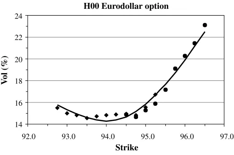
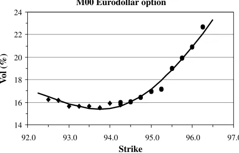
Let us apply SABR to options on US dollar interest rates. There are three key groups of European options on US rates: Eurodollar future options, caps/floors, and European swaptions. Eurodollar future options are exchange-traded options on the 3 month Libor rate; like interest rate futures, EDF options are quoted on 100(1−rL i b o r). Figure 1.1 fits the
SABR model (with β=1) to the implied volatility for the June 99 con-tracts, and figures 3.4–3.7 fit the model (also with β=1) to the implied volatility for the September 99, December 99, and March 00 contracts. All prices were obtained from Bloomberg Information Services on March 23, 1999. Two points are shown for the same strike where there are quotes for both puts and calls. Note that market liquidity dries up for the later contracts, and for strikes that are too far from the money. Consequently, more market noise is seen for these options.
Caps and floors are sums of caplets and floorlets; each caplet and floorlet is a European option on the 3 month Libor rate. We do not con-sider the cap/floor market here because the broker-quoted cap prices must be “stripped” to obtain the caplet volatilities before SABR can be applied.
A m year into n yearswaption is a European option with m years to the exercise date (the maturity); if it is exercised, then one receives an n year swap (the tenor, or underlying) on the 3 month Libor rate. See Appendix A. For almost all maturities and tenors, the US swaption market is liquid for at-the-money swaptions, but is ill-liquid for swaptions struck away from the money. Hence, market data is somewhat suspect for swaptions that are not struck near the money. Figures 3.8–3.11 fits the SABR model (with β=1) to the prices of m into5Yswaptions observed on April 28, 2000. Data supplied courtesy of Cantor-Fitzgerald.
We observe that the smile and skew depend heavily on the time-to-exercise for Eurodollar future options and swaptions. The smile is pro-nounced for short-dated options and flattens for longer dated options;
the skew is overwhelmed by the smile for short-dated options, but is important for long-dated options. This picture is confirmed tables 3.1 and 3.2. These tables show the values of the vol of vol νand correlation ρ
obtained by fitting the smile and skew of each “m into n” swaption, again using the data from April 28, 2000. Note that the vol of vol νis very high for short dated options, and decreases as the time-to-exercise increases, while the correlations starts near zero and becomes substan-tially negative. Also note that there is little dependence of the market skew/smile on the length of the underlying swap; both νand ρare fairly constant across each row. This matches our general experience: in most markets there is a strong smile for short-dated options which relaxes as the time-to-expiry increases; consequently the volatility of volatility ν is large for short dated options and smaller for long-dated options, regard-less of the particular underlying. Our experience with correlations is regard-less clear: in some markets a nearly flat skew for short maturity options develops into a strongly downward sloping skew for longer maturities. In other markets there is a strong downward skew for all option maturities, and in still other markets the skew is close to zero for all maturities.
U99 Eurodollar option
10 15 20 25 30
93.0 94.0 95.0 96.0 97.0
Strike
V
ol (%)
Fig.3.4 Volatility of the Sep 99 EDF options
Strike
V
ol (%)
Z99 Eurodollar option
14 16 18 20
92.0 93.0 94.0 95.0 96.0
Fig. 3.5 Volatility of the Dec 99 EDF options
V
ol (%)
14 16 18 20 22 24
92.0 93.0 94.0 95.0 96.0 97.0
Strike H00 Eurodollar option
^
3.2. Managing smile risk. After choosing β and fitting ρ, ν, and either αor σATM, the SABR model
dFˆ= ˆαFˆβdW
1, Fˆ(0)=f (3.4a)
dαˆ =ναˆdW2, α(ˆ 0)=α (3.4b)
with
dW1dW2=ρdt (3.4c)
fits the smiles and skews observed in the market quite well, especially considering the quality of price quotes away from the money . Let us take for granted that it fits well enough. Then we have a single, self-consistent model that fits the option prices for all strikes Kwithout “adjustment,” so we can use this model to price exotic options without ambiguity. The SABR model also predicts that whenever the forward price fchanges, the the implied volatility curve shifts in the samedirection and by the same
amount as the price f. This predicted dynamics of the smile matches market experience. If β <1, the “backbone” is downward sloping, so the shift in the implied volatility curve is not purely horizontal. Instead, this curve shifts up and down as the at-the-money point traverses the back-bone. Our experience suggests that the parameters ρ and ν are very sta-ble (βis assumed to be a given constant), and need to be re-fit only every few weeks. This stability may be because the SABR model reproduces the usual dynamics of smiles and skews. In contrast, the at-the-money volatility σATM, or, equivalently, α may need to be updated every few hours in fast-paced markets.
Since the SABR model is a single self-consistent model for all strikes K, the risks calculated at one strike are consistent with the risks calculated at other strikes. Therefore the risks of all the options on the same asset can be added together, and only the residual risk needs to be hedged.
Let us set aside the risk for the moment, and calculate the other risks. Let BS(f,K, σB,tex) be Black’s formula (2.4a–2.4c) for, say, a call
option. According to the SABR model, the value of a call is
Vcall=BS(f,K, σB(K,f),tex) (3.5)
where the volatility σB(K,f)≡σB(K,f;α, β, ρ , ν ) is given by equations (2.17a–2.17c). Differentiating @ footnote:{In practice risks are calculated by finite differences: valuing the option at α, re-valuing the option after
V
ol (%)
M00 Eurodollar option
14 16 18 20 22 24
92.0 93.0 94.0 95.0 96.0 97.0
Strike
Fig, 3.7 Volatility of the Jun 00 EDF options
3M into 5Y
12% 14% 16% 18% 20%
4% 6% 8% 10% 12%
Fig. 3.8 Volatilities of 3 month into 5 year swaption
1Y into 5Y
13% 14% 15% 16% 17% 18%
4% 6% 8% 10% 12%
Fig. 3.9 Volatilities of 1 year into 1 year swaptions
5Y into 5Y
12% 13% 14% 15% 16% 17%
4% 6% 8% 10% 12%
bumping the forward to α+δ, and then subtracting to determine the risk This saves differentiating complex formulas such as (2.17a–2.17c). with respect to α yields the vega risk, the risk to overall changes in volatility:
∂Vcall
∂α =
∂BS
∂σB·
∂σB(K,f;α, β, ρ , ν )
∂α . (3.6)
This risk is the change in value when αchanges by a unit amount. It is traditional to scale vega so that it represents the change in value when the ATM volatility changes by a unit amount. Since δσATM =(∂ σATM/∂ α ) δα, the vega risk is
vega≡ ∂Vcall
∂α =
∂BS
∂σB ·
∂ σB(K,f;α,β ,ρ ,ν )
∂ α ∂ σATM(f;α,β ,ρ ,ν )
∂ α
(3.7a)
where σATM(f)=σB(f,f) is given by (2.18). Note that to leading order,
∂σB/∂ α≈σB/α and ∂σATM/∂ α≈σATM/α, so the vega risk is roughly given by
vega≈ ∂BS
∂σB ·
σB(K,f) σATM(f) =
∂BS
∂σB ·
σB(K,f)
σB(f,f). (3.7b)
Qualitatively, then, vega risks at different strikes are calculated by bump-ing the implied volatility at each strike Kby an amount that is propor-tional to the implied volatiity σB(K,f) at that strike. That is, in using equation (3.7a), we are essentially using proportional, and not parallel, shifts of the volatility curve to calculate the total vega risk of a book of options.
Since ρ and ν are determined by fitting the implied volatility curve observed in the marketplace, the SABR model has risks to ρand ν
changing. Borrowing terminology from foreign exchange desks, vanna is the risk to ρ changing and volga (vol gamma) is the risk to νchanging:
vanna=∂Vcall
∂ρ =
∂BS
∂σB ·
∂σB(K,f;α, β, ρ , ν )
∂ρ , (3.8a)
volga= ∂Vcall
∂ν =
∂BS
∂σB ·
∂σB(K,f;α, β, ρ , ν )
∂ν . (3.8b)
Vanna basically expresses the risk to the skew increasing, and volga expresses the risk to the smile becoming more pronounced. These risks are easily calculated by using finite differences on the formula for σB in equations (2.17a–2.17c). If desired, these risks can be hedged by buying or selling away-from-the-money options.
10Y into 5Y
9% 10% 11% 12% 13%
4% 6% 8% 10% 12%
Fig. 3.11 Volatilities of 10 year into 5 year options
1Y 2Y 3Y 4Y 5Y 7Y 10Y
1M 76.2% 75.4% 74.6% 74.1% 75.2% 73.7% 74.1% 3M 65.1% 62.0% 60.7% 60.1% 62.9% 59.7% 59.5% 6M 57.1% 52.6% 51.4% 50.8% 49.4% 50.4% 50.0% 1Y 59.8% 49.3% 47.1% 46.7% 46.0% 45.6% 44.7% 3Y 42.1% 39.1% 38.4% 38.4% 36.9% 38.0% 37.6% 5Y 33.4% 33.2% 33.1% 32.6% 31.3% 32.3% 32.2% 7Y 30.2% 29.2% 29.0% 28.2% 26.2% 27.2% 27.0% 10Y 26.7% 26.3% 26.0% 25.6% 24.8% 24.7% 24.5%
TABLE 3.1
VOLATILITY OF VOLATILITY
ν
FOR EUROPEAN
SWAPTIONS. ROWS ARE TIME–TO–EXERCISE;
COLUMNS ARE TENOR OF THE UNDERLYING SWAP.
1Y 2Y 3Y 4Y 5Y 7Y 10Y
1M 4.2% –0.2% –0.7% –1.0% –2.5% –1.8% –2.3% 3M 2.5% –4.9% –5.9% –6.5% –6.9% –7.6% –8.5% 6M 5.0% –3.6% –4.9% –5.6% –7.1% –7.0% –8.0% 1Y –4.4% –8.1% –8.8% –9.3% –9.8% –10.2% –10.9% 3Y –7.3% –14.3% –17.1% –17.1% –16.6% –17.9% –18.9% 5Y –11.1% –17.3% –18.5% –18.8% –19.0% –20.0% –21.6% 7Y –13.7% –22.0% –23.6% –24.0% –25.0% –26.1% –28.7% 10Y –14.8% –25.5% –27.7% –29.2% –31.7% –32.3% –33.7%
TABLE 3.2
^
The delta risk expressed by the SABR model depends on whether one uses the parameterization α, β, ρ, νor σATM, β, ρ, ν. Suppose first we use the parameterization α, β, ρ, ν, so that σB(K,f)≡σB(K,f;α, β, ρ , ν ). Differentiating respect to f yields the risk
≡∂Vcall
∂f =
∂BS
∂f +
∂BS
∂σB
∂σB(K,f;α, β, ρ , ν )
∂f . (3.9)
The first term is the ordinary risk one would calculate from Black’s model. The second term is the SABR model’s correction to the risk. It consists of the Black vega times the predictedchange in the implied volatil-ity σBcaused by the change in the forward f. As discussed above, the pre-dicted change consists of a sideways movement of the volatility curve in the same direction (and by the same amount) as the change in the for-ward price f. In addition, if β <1the volatility curve rises and falls as the at-the-money point traverses up and down the backbone. There may also be minor changes to the shape of the skew/smile due to changes in f.
Now suppose we use the parameterization σAMT, β, ρ, ν. Then αis a function of σATM and fdefined implicitly by (2.18). Differentiating (3.5) now yields the risk
≡∂BS
∂f +
∂BS
∂σB
∂σ
B(K,f;α, β, ρ , ν )
∂f +
∂σB(K,f;α, β, ρ , ν ) ∂α
∂α(σATM,f) ∂f
.
(3.10) The delta risk is now the risk to changes in f with σATM held fixed. The last term is just the change in αneeded to keep σATM constant while f changes. Clearly this last term must just cancel out the vertical compo-nent of the backbone, leaving only the sideways movement of the implied volatilty curve. Note that this term is zero for β=1.
Theoretically one should use the from equation (3.9) to risk man-age option books. In many markets, however, it may take several days for volatilities σB to change following significant changes in the forward price f. In these markets, using from (3.10) is a muchmore effective hedge. For suppose one used from equation (3.9). Then, when the volatility σATM did not immediately change following a change in f, one would be forced to re-mark αto compensate, and this re-marking would change the hedges. As σATM equilibrated over the next few days, one would mark α back to its original value, which would change the
hedges back to their original value. This “hedging chatter” caused by market delays can prove to be costly.
Appendix A. Analysis of the SABR Model
Here we use singular perturbation techniques to price European options under the SABR model. Our analysis is based on a small volatility expan-sion, where we take both the volatility αˆ and the “volvol” νto be small. To carry out this analysis in a systematic fashion, we re-write αˆ −→εα,ˆ andν−→εν, and analyze
dFˆ=εαˆC(Fˆ)dW1, (A.1a)
dαˆ =εναˆdW2, (A.1b)
with
dW1dW2=ρdt, (A.1c)
in the limit ε1. This is the distinguished limit[21], [22] in the language of singular perturbation theory. After obtaining the results we replace
εαˆ −→ ˆα,and εν−→ν to get the answer in terms of the original vari-ables. We first analyze the model with a general C(Fˆ), and then specialize the results to the power law Fˆβ. This is notationally simpler than working
with the power law throughout, and the more general result may prove valuable in some future application.
We first use the forward Kolmogorov equation to simplify the option pricing problem. Suppose the economy is in state Fˆ(t)=f, α(ˆ t)=α at date t. Define the probability density p(t,f, α;T,F,A)by
p(t,f, α;T,F,A)dF dA=probF<Fˆ(T) <F+dF, A<α(ˆ T) <A+dAFˆ(t)=f, α(ˆ t)=α.
(A.2)
As a function of the forward variables T,F,A,the density psatisfies the for-ward Kolmogorov equation (the Fo˝kker-Planck equation)
pT=12ε
2A2[C2(F)p]
FF +ε2ρν[A2C
(F)p]FA+12ε 2
ν2[A2p]
A A forT>t,
(A.3a)
with
p=δ(F−f) δ(A−α ) atT=t, (A.3b)
as is well-known [24], [25], [26]. Here, and throughout, we use subscripts to denote partial derivatives.
Let V(t,f, α )be the value of a European call option at date t, when the economy is in state Fˆ(t)=f, α(ˆ t)=α.Let texbe the option’s exercise date,
and let Kbe its strike. Omitting the discount factor D(tset), which factors
out exactly, the value of the option is
V(t,f, α )=E
[Fˆ(tex)−K]+| ˆF(t)=f, α(ˆ t)=α
=
∞
−∞
∞
K
(F−K )p(t,f, α;tex,F,A)dF dA.
See (2.1a). Since
p(t,f, α;tex,F,A)=δ(F−f) δ(A−α )+
tex
t
pT(t,f, α;T,F,A)dT, (A.5) we can re-write V(t,f, α )as
V(t,f, α )=[f−K]++
tex
t
∞
K
∞
−∞
(F−K)pT(t,f, α;T,F,A)dA dF dT.
(A.6) We substitute (A.3a) for pT into (A.6). Integrating the A derivatives ε2ρν[A2C(F)p]
FA and 12ε 2ν2[A2p]
A A over all A yields zero. Therefore our
option price reduces to
V(t,f, α )=[f−K]++1 2ε
2 tex
t
∞
−∞
∞
K
A2(F−K )[C2(F)p]
FFdF dA dT,
(A.7)
where we have switched the order of integration. Integrating by parts twice with respect to Fnow yields
V(t,f, α )=[f−K]++1 2ε
2C2(K) tex
t
∞
−∞
A2p(t,f, α;T,K,A)dA dT. (A.8)
The problem can be simplified further by defining P(t,f, α;T,K)=
∞
−∞
A2p(t,f, α;T,K,A)dA. (A.9)
Then Psatisfies the backward’s Kolmogorov equation [24], [25], [26] Pt+
1 2ε
2α2C2(f)P
ff+ε2ρνα2C(f)Pfα+
1 2ε
2ν2α2P
αα =0, fort<T
(A.10a)
P=α2δ(f−K), fort=T. (A.10b)
Since tdoes not appear explicitly in this equation, Pdepends only on the combination T−t, and not on tand Tseparately. So define
τ =T−t, τex=tex−t. (A.11)
Then our pricing formula becomes
V(t,f, α )=[f−K]++1 2ε
2C2(K) τex
0
P(τ,f, α;K)dτ (A.12)
where P(τ,f, α;K) is the solution of the problem
Pτ =
1 2ε
2α2C2(f)P
ff+ε2ρνα2C(f)Pfα+
1 2ε
2ν2α2P
αα, forτ >0, (A.13a)
P=α2δ(f−K), forτ=0. (A.13b)
In this appendix we solve (A.13a), (A.13b) to obtain P(τ,f, α;K), and then substitute this solution into (A.12) to obtain the option value V(t,f, α ). This yields the option price under the SABR model, but the resulting formulas are awkward and not very useful. To cast the results in a more usable form, we re-compute the option price under the normal model
dFˆ=σNdW, (A.14a)
and then equate the two prices to determine which normal volatility σN
needs to be used to reproduce the option’s price under the SABR model. That is, we find the “implied normal volatility” of the option under the SABR model. By doing a second comparison between option prices under the log normal model
dFˆ=σBF dWˆ (A.14b) and the normal model, we then convert the implied normal volatility to the usual implied log-normal (Black-Scholes) volatility. That is, we quote the option price predicted by the SABR model in terms of the option’s implied volatility.
A.1 Singular perturbation expansion. Using a straightforward per-turbation expansion would yield a Gaussian density to leading order,
P= α
2π ε2C2(K) τe
− (f−K)2
2ε2α2C2(K) τ{1+ · · ·}. (A.15a)
Since the “+ · · ·” involves powers of (f−K) /εαC(K),this expansion would become inaccurate as soon as (f−K)C(K) /C(K)becomes a sig-nificant fraction of 1; i.e., as soon as C(f)and C(K)are significantly dif-ferent. Stated differently, small changes in the exponent cause much greater changes in the probability density. A better approach is to re-cast the series as
P= α
2π ε2C2(K) τe
− (f−K)2
2ε2α2C2(K) τ{1+···} (A.15b)
^
Suppose we define the new variable
z= 1
so that the solution Pis essentially e−z2/2. To leading order, the density is
Gaussian in the variable z, which is determined by how “easy” or “hard” it is to diffuse from Kto f, which closely matches the underlying physics. The fact that the Gaussian changes by orders of magnitude as z2 increases should be largely irrelevent to the quality of the expansion.
This approach is directly related to the geometric optics technique that is so successful in wave propagation and quantum electronics [27], [22]. To be more specific, we shall use the near identity transform method to carry out the geometric optics expansion. This method, pioneered in [28], transforms the problem order-by-order into a simple canonical problem, which can then be solved trivially. Here we obtain the solution only through O(ε2), truncating all higher order terms.
Let us change variables from fto z= 1
and to avoid confusion, we define
B(εαz)=C(f) . (A.18b)
Therefore, (A.12) through (A.13b) become
V(t,f,a)=[f−K]++1 To leading order Pˆis the solution of the standard diffusion problem
ˆ
Pτ= 12Pˆzz with Pˆ=δ(z)at τ =0. So it is a Gaussian to leading order. The
next stage is to transform the problem to the standard diffusion prob-lem through O(ε ), and then through O(ε2), . . .. This is the near
Note that the variable αdoes not enter the problem for Pˆuntil O(ε ), so
ˆ
P(τ,z, α )= ˆP0(τ,z)+ ˆP1(τ,z, α )+ · · · (A.25)
Consequently, the derivatives Pˆzα, Pˆαα, and Pˆαare all O(ε ). Recall that we
are only solving for Pˆ through O(ε2). So, through this order, we can
re-write our problem as
ˆ Let us now eliminate the 1
2εa(B/B)Pˆzterm. Define H(τ,z, α )by The option price now becomes
V(t,f,a)=[f−K]++1 Equations (A.30a), (A.30b) are independent of αto leading order, and at O(ε )they depend on αonly through the last term ερνα(Hzα+12εα
B B;Hα).
As above, since A.30a is independent of αto leading order, we can con-clude that theαderivatives Hα and Hzα are no larger than O(ε ), and so
the last term is actually no larger than O(ε2). Therefore His independent
of αuntil O(ε2)and the αderivatives are actually no larger than O(ε2).
Thus, the last term is actually only O(ε3), and can be neglected since we
are only working through O(ε2). So, There are no longer any αderivatives, so we can now treat αas a parame-ter instead of as an independent variable. That is, we have succeeded in effectively reducing the problem to one dimension.
Let us now remove the Hz term through O(ε2). To leading order,
B(εαz) /B(εαz)and B(εαz) /B(εαz)are constant. We can replace these ratios by
b1=B(εαz0) /B(εαz0), b2=B(εαz0) /B(εαz0), (A.32)
commiting only an O(ε )error, where the constant z0will be chosen later.
We now define Hˆby
H=eε2ρ ν αb
1z2/4Hˆ. (A.33)
Then our option price becomes V(t,f,a)=[f−K]++1 We’ve almost beaten the equation into shape. We now define
x= 1
which can be written implicitly as
^
In terms of x, our problem is V(t,f,a)=[f−K]++1
The final step is to define Qby
ˆ
where Qis the solution of
Qτ =
The solution of A.45a, A.45b is clearly
Q= √1
This solution yields the option price V(t,f,a)=[f−K]++1
Observe that this can be written as V(t,f,a)=[f−K]++1
That is, the value of a European call option is given by
A.2. Equivalent normal volatility. Equations (A.52a) and (A.52a) are a formula for the dollar price of the call option under the SABR model. The utility and beauty of this formula is not overwhelmingly apparent. To obtain a useful formula, we convert this dollar price into the equiva-lent implied volatilities. We first obtain the implied normalvolatility, and then the standard log normal(Black) volatility.
Suppose we repeated the above analysis for the ordinary normal model dFˆ=σNdW, Fˆ(0)=f. (A.53a) where the normal volatily σNis constant, not stochastic. (This model is also called the absoluteor Gaussianmodel). We would find that the option value for the normal model is exactly
V(t,f)=[f−K]++|f−K| A.52a, A.52b. Working out this integral then yields the exact European option price for the normal model, where N is the normal distribution and Gis the Gaussian density matches the option price under the SABR model A.52a, A.52a if and only if we choose the normal volatility σNto be
1
Taking the square root now shows the option’s implied normal (absolute) volatilityis given by
σN=
Before continuing to the implied log normalvolatility, let us seek the simplest possible way to re-write this answer which is correct through
This factor represents the average difficulty in diffusing from today’s for-ward f to the strike K, and would be present even if the volatility were not stochastic.
The next factor is z
f Kis the geometric average of fand K. (The arithmetic aver-age could have been used equally well at this order of accuracy). This fac-tor represents the main effect of the stochastic volatility.
The coefficients φ1, φ2, and φ3provide relatively minor corrections.
Through O(ε2)these corrections are
^
Let us briefly summarize before continuing. Under the normal model, the value of a European call option with strike Kand exercise date τexis given by (A.54a), (A.54b). For the SABR model,
dFˆ=εαˆC(Fˆ)dW1, Fˆ(0)=f (A.58a)
dαˆ =εναˆdW2, α(ˆ 0)=α (A.58b)
dW1dW2=ρdt, (A.58c)
the value of the call option is given by the same formula, at least through O(ε2), provided we use the implied normal volatility
σN(K)= εα(ff−K)
The first two factors provide the dominant behavior, with the remaining factor 1+[· · ·]ε2τ
exusually provideing corrections of around 1% or so.
One can repeat the analysis for a European put option, or simply use call/put parity. This shows that the value of the put option under the traders prefer to quote prices in terms of Black (log normal) volatilities, rather than normal volatilities. To derive the implied Black volatility, consider Black’s model
dFˆ=εσBFdWˆ , Fˆ(0)=f, (A.61)
where we have written the volatility as εσB to stay consistent with the preceding analysis. For Black’s model, the value of a European call with strike Kand exercise date τexis
Vcall =fN(d1)−KN(d2), (A.62a)
where we are omitting the overall factor D(tset)as before.
We can obtain the implied normal volatility for Black’s model by repeating the preceding analysis for the SABR model with C(f)=fand
ν=0. Setting C(f)=fand ν=0in (A.59a – A.59c) shows that the
nor-volatility for Black’s model is
σN(K)=εσBf K 1+
A.4. Stochastic βmodel. As originally stated, the SABR model
con-Making this substitution in (A.58a–A.58b) shows that the implied normal volatility for this model is
σN(K)=
We can simplify this formula by expanding
f−K=f Klogf/K
and neglecting terms higher than fourth order. This expansion reduces the implied normal volatility to
σN(K)=εα(f K This is the formula we use in pricing European calls and puts.
To obtain the implied Black volatility, we equate the implied normal volatility σN(K) for the SABR model obtained in (A.69a – A.69b) to the implied normal volatility for Black’s model obtained in (A.63). This shows that the implied Black volatility for the SABR model is
σB(K)= εα
from setting εto 1 to recover the original units, this is the formula quot-ed in section 2, and fittquot-ed to the market in section 3.
A.5. Special cases Two special cases are worthy of special treatment: the stochastic normal model (β=0) and the stochastic log normal model (β=1). Both these models are simple enough that the expansion can be continued through O(ε4). For the stochastic normalmodel (β=0)
the implied volatilities of European calls and puts are
σN(K)=εα
For the stochastic log normal model (β=1)the implied volatilities are